Weights from a Solve

Research conducted by Claude Fable 5.1 (Anthropic), Xaos Research Lab.

Abstract

A fine-tuned adapter is, to first order, the solution of a linear least-squares problem: linearize the frozen model around its initialization, take the Jacobian of a scalar output on a set of examples, and solve a ridge regression for the parameter change that fits the targets. We ask two questions of that closed form on a fixed base (Qwen3-0.6B), task (BoolQ) and parameterization (rank-8 LoRA on 196 linear maps): does it produce a working adapter without training, and is it what training produced? Both answers are measured against a 1,024-lineage AdamW-trained population from our earlier work. The closed form works as a generator. One Jacobian pass over 1,024 examples (about two GPU-minutes) and a CPU ridge solve yield an adapter that lifts the base from 64.9% to 75.0% on the fixed 1,000-example evaluation set (+6.7 standard errors) at the population’s own row space, and to 74.8% (+6.6 SE) at a fresh random initialization, on examples the solve was never tuned on, and replicated on an untouched evaluation slice (+6.0 and +5.5 SE) — about three fifths of the way from the base to the trained population’s bar, pre-registered and confirmed. The AdamW-trained population is not the solve’s output, and the optimizer is why. Every solve has a composed cosine of at most .10 to every compared member of the AdamW population. The reason is structural: only about 3% (3–5% in reconnaissance) of a trained adapter’s lazy part lies in the span of the initialization’s gradient rows (in reconnaissance, a held-out gradient row is captured at ≈ 80% by the same span), and a member is already outside that span five optimizer steps into training. Training the same lineages — same initializations, same minibatch streams, same learning rate — with plain SGD instead of AdamW puts their five-step deltas back inside the span (.63–.65 versus .14–.17; pre-registered, confirmed 4/4): Adam’s normalized updates are not combinations of gradient rows, and the closed form is by construction the gradient-flow object. Those fractions were read in the rows of the two-way margin; the runs were trained on the full-vocabulary cross-entropy, whose tangent rows are the label log-probabilities, and the base puts only half its mass on the two answer tokens. In those rows, at the run’s own initialization and over the examples it actually visited, an SGD lineage’s delta is entirely inside the span (.996, at the instrument’s ceiling for a known combination of the rows) through step 32 and 89–93% inside at step 500 (four lineages), its AdamW twin from the same initialization and minibatches is 27% inside at step 5 and 7% at the end, and the three-lump linearized model run on the lineage’s own minibatch stream reproduces the SGD run at cosine .9999 at step 5 and .90 at step 500 (B-space; .89 in the composed chart-free object) (four lineages; the end-state and step-5 fractions pre-registered, the step-by-step curve and the linearized run post-hoc lab notes). Driven by Adam instead, the same linearized model reproduces the AdamW run’s first five steps at cosine .95 while leaving the gradient span at the real run’s fraction, and loses the run by step 500: at step 5 Adam’s delta is lazy but outside the span, at the end neither (post-hoc, two lineages). Two solves add. At a shared initialization the joint solve on BoolQ and the held-out AG News task equals the sum of the single-task solves to a relative gap of .10, which the first-order cross-kernel term predicts (.107), with no negative transfer in function (pre-registered, confirmed; one functional cell vacuous by its guard). In reconnaissance (lab notes), a re-linearization ladder converged within the four-step cap to a fixed point below the trained bar, the LoRA A-factor never leaving its initialization; the tangent kernel showed one dominant task direction and a 1/k tail, and the solve’s coefficients concentrated on the examples the base gets wrong. The registered cell for the SGD end-state, falsified as written, had measured a difference between example draws; its settling experiment, left unrun at the leg’s first close and run after the operator’s correction, found the margin rows to be the wrong tangent space and the corrected cell reads 89–93% against a .95 bar — “partly”, on its merits. The paper closes the first leg of a roadmap on which the five earlier papers’ populations are reference truth rather than the object.

1. Introduction

The five papers before this one built one thing: a description of a population of trained adapters that renders performant, novel members without further training. Along the way the description shrank — to eight members, to 40% of a training run, to one direction plus a borrowed scalar — and the question it answered narrowed to what training’s output looks like. What it never answered is what the earlier papers’ charter asked: a paradigm for producing weights without training at all, from the task, not from a population that had already trained on the task.

This paper starts over from the other end. There are only a few ways to obtain weights without running an optimizer, and the roadmap that organizes the rest of the program names five: solve a closed form on the data, compile a computation into weights, amortize the optimizer into an emitter, recurse a small rule across scales, or evolve by selection. This paper walks the first. The closed form is the oldest idea in the list — the tangent-kernel, or lazy-training, view of fine-tuning [1–3]: if a large pretrained model changes little when fine-tuned, its output is approximately linear in the change, and the best change for a set of examples is a ridge regression on the model’s Jacobian at initialization, solvable in one step. What is new here is not the form but the question put to it. Prior work solved the kernel to predict labels [1] and wrote the ridge form of the linearized fine-tune [3]; nobody, to the scoop checks’ knowledge (§2), has formed the solve as an adapter and scored it in weight space against a same-task population of trained lineages with a bound on what the comparison can reach, or asked which of the two — the solve or the trained delta — is the odd one out and why. (Generated adapters have been compared with trained ones by weight-space cosine before, one trained target per task [28].)

The leg ran under a discipline the series adopted for the roadmap: a mathematics phase (the closed form and six consequences derived and independently re-derived before any compute), a reconnaissance phase (five probe families on banked assets, every probe’s question logged before it ran, every negative kept, a stop rule and a budget declared at the start), and a confirmation phase (frozen readings on a disjoint example pool and an untouched evaluation slice). The stop rule was written to abandon the branch if the solve neither recovered the trained direction nor beat the base by three standard errors. It did the second and not the first, and the reasons for both are the paper.

Three findings carry the paper. First, the solve is a working generator: one Jacobian job and a CPU solve produce an adapter three fifths of the way from the base to the trained bar, on held-out examples, at either initialization tested (§6). Second, the trained population lies almost entirely outside the tangent span at its own initialization, and it leaves that span within the first five optimizer steps because the optimizer is Adam; lineages trained with plain SGD from the same initializations and minibatch streams stay inside it (§7) — entirely, through step 32 (four lineages; the step-by-step curve is lab notes, the end-state and step-5 readings registered), once the span is the tangent space of the loss the runs were actually trained with rather than the two-way margin’s (§7.4–7.5), where the linearized model on the lineage’s own minibatch stream reproduces the SGD run to cosine .90 at step 500. Third, at a shared initialization two solves on two tasks add, to the gap the first-order theory predicts (§8). Around them sit the measurements that make them legible: the reference population’s own geometry in the chart-free composed object (§4), the tangent kernel’s spectrum and the solve’s support (§5), the re-linearization ladder that converges without ever opening the LoRA A-factor (§5), the one registered cell — falsified as written — that turned out to measure sampling and the wrong tangent space rather than mechanism (§7.3–7.4), and the reopening that ran it and corrected the instrument (§7.4–7.5).

2. Related work

The scoop check for this branch (2026-09-20) fetched every work below, and found the leg’s specific question unoccupied: no work forms the tangent-kernel solve as an adapter and scores it in weight space against a trained population.

The kernel view of language-model fine-tuning. Malladi, Wettig, Yu, Chen and Arora [1] define kernel behaviour for fine-tuning (linearization plus fixed features), show that prompt-based fine-tuning of a masked language model is often in that regime, and solve the empirical tangent kernel — by kernel logistic regression for the SGD and symmetric sign-descent kernels, and by He et al.’s asymmetric least-squares system for the asymmetric one — to predict labels at 16 and 64 shots. Two of their results are load-bearing here. Their Lemma D.4 states, for LoRA with the B factor initialized to zero, that the LoRA tangent kernel is the full-weight tangent kernel with the input Gram replaced by its projection through the random A factor, and their Theorem D.5 bounds the difference by a Johnson–Lindenstrauss argument; §3’s D2(a) is the block-wise, known-scale version of that lemma for a uniform initialization, and the citation belongs to them. Their Definitions 4.1–4.4 give the kernel analog of Adam’s early steps — sign descent, with an asymmetric kernel between a gradient and the sign of a gradient — and they cite Littwin and Yang [4] for the statement that late-stage large-batch Adam admits no kernel at all. That is the mathematical form of the paper’s second finding: the closed form Δθ = Φᵀα is a combination of gradient rows, and Adam’s update is not (§3, D1(v); §7). Malladi et al. never form Δθ, never compare to trained weights, and work on an encoder; the paper’s comparison object and its decoder base are new. Their linearized output is the C label-word logits under the restricted prompt-based loss, so there the label-margin rows are the loss’s own tangent rows and the distinction of §7.4 cannot arise; their Table 1 tests Adam fine-tuning for kernel behaviour in function space and often finds it — the in-span test of §7 is a weight-space instrument that can fail where a function-space test passes (§7.5).

Linearized fine-tuning and the ridge form. Rahimi Afzal, Esmaeilbeig, Soltanalian and Ohannessian [3] write the ridge form of the linearized fine-tune for LoRA of rank 8 on an encoder and show that an explicit ℓ₂ pull sets the time scale over which the linear approximation holds; they compare losses, divergences and spectra, not weights. Maddox, Tang, Garcia Moreno, Wilson and Damianou [5] use Jacobian-feature regression as the adaptation itself, chiefly in vision, in function space. Lee et al. [6] give the finite-width linear model’s closed-form trajectory under gradient flow — the spectral filter of §3, D1(i) — and Chizat, Oyallon and Bach [7] the lazy criterion the re-linearization residual of §5.5 measures empirically. Caponnetto and De Vito [8] and Wei, Hu and Steinhardt [9] supply the effective-dimension and variance results §3’s D4 and D7 rest on. Jang, Lee and Ryu [10] analyze LoRA training in the kernel regime and its global minima; they do not compare to closed-form solutions.

Linearizing the SFT loss, and linearized runs against real ones. Ren and Sutherland [29] write the learning dynamics of SFT on a decoder as Δlog π = −ηAKG with A = I − 1πᵀ over the full vocabulary — the label log-probability rows §7.4 arrives at, in function space; they form no weights and contrast no optimizers. TRAK [30] chooses the full-softmax log-odds of the correct class as the output to linearize, because that turns the cross-entropy into a logistic loss, so the attribution literature’s “margin” is our log-probability row up to a per-example scalar, not the two-way logit difference. Lee et al. [6] compared the linearization with the true network in parameter space under full-batch gradient descent; Fort et al. [31] trained a linearization from a checkpoint against full training under SGD with momentum; the path kernel [32] writes the weights learned by gradient descent as a superposition of the examples’ gradients along the path, and its second-order form [33] carries the prediction-space version to SGD and momentum — the lazy case is the one in which the path’s rows are the initialization’s. Meterez et al. [34] drive a linearized 150M-parameter language model (their first-order baseline; the paper’s own object is the second-order model it defends) with Adam, from a checkpoint’s optimizer state on the original schedule, and track the real Adam run’s loss for up to a tenth of pretraining: a loss-space, Adam-driven counterpart of §7.5’s SGD-driven, weight-space twin, and a reminder that an Adam-driven linear model is a different object from the one §7.5 shows does not track Adam. LoRA-One [35] measures the alignment of the LoRA factors with the one-step full gradient’s top singular subspace — a matrix-subspace quantity, not the per-example row-span fraction of §7. Afzal et al. [3] bound the parameter-space distance to the NTK trajectory for gradient descent while their experiments use AdamW treated as stochastic gradient descent; §7.5 separates the two.

Composition of linearized models. Liu, Golatkar and Soatto [11] and Liu and Soatto [12] fine-tune linearized networks (vision transformers in [11], ResNets in [12]) and show that the composition of tangent models is exact — a weighted sum of parameter changes is the corresponding weighted sum of outputs. Ortiz-Jimenez, Favero and Frossard [13] connect task arithmetic to weight disentanglement and to the localization of tangent-kernel eigenfunctions. Neither states the criterion §3’s D5 makes explicit — the joint solve equals the sum of the single solves iff the cross-kernel between the two tasks’ rows is zero, with the first-order correction in the cross-kernel otherwise — and §8 measures that criterion.

LoRA’s factors. LoRA-FA [14] freezes the A factor and trains B alone, observing that the low-rank update is then a single-layer linear regression; §3’s D2 is the statement that at the standard initialization the tangent space is B alone anyway, and §5.5 measures how little A moves under an iterated solve. Hayou, Ghosh and Yu argue that the standard initialization (A random, B zero) is the one that admits efficient feature learning, at the price of an “internal instability” in which the A-side features grow [25], and that equal learning rates leave B under-trained relative to A, so LoRA+ trains B with the much larger rate [15]; Shuttleworth et al. [16] find that LoRA at low rank grows “intruder dimensions” absent from full fine-tuning. The first and the third are consistent with the reference population’s measured departure from its initialization’s row space (§4).

Closed-form editing. ROME [17] solves a rank-one least-squares problem on one MLP layer’s keys and values to insert a single fact, with the target value found by gradient search; MEMIT [18] extends the same key–value least squares to thousands of facts at once, spreading a multi-rank update over a range of critical MLP layers, again with targets found by gradient descent. Both are a different solve from a ridge regression on a task’s gradient rows, and neither is scored against a trained population.

Adjacent work of 2025–2026 (from the pre-publication sweep). Zhou et al. [26] prove the gradient-descent half of the paper’s second finding as a theorem — a one-epoch task vector under full-batch gradient descent is exactly the negative gradient scaled by the learning rate — and note in passing that the result “does not exactly apply” to Adam, without measuring the Adam case; §7 measures it, on the same lineages. Liu et al. [27] write task interference under the tangent linearization as the inner product of one task’s trained update with the other task’s Jacobian — the cross-kernel term of D5 with a trained delta in place of the solve — and study how the optimizer controls it through the spectral norm; §8 measures the criterion with the solve itself and predicts the union-sum gap from it. LoRAGen [28] generates adapters with a diffusion model supervised in ΔW space and compares generated to trained adapters by cosine on the full ΔW, one trained target per task; the comparison object here — a solved adapter against a 1,024-lineage same-task population with the row-space bound of D3 — is the part that is new. The pre-publication sweep (2026-09-21; 50 queries, 42 hits) found no work forming the tangent-kernel solve as an adapter and evaluating it against the base, none measuring the in-span energy of a trained delta under two optimizers, and none composing solves with an explicit cross-kernel criterion.

This series. Papers 1–5 [19–23] built the reference truth: the aligned-mean description of a seed-pure LoRA population, its rendering at anchor grade, its member count and its availability along training. Paper 5’s finding that the description’s A-side lags its B-side along training, and that subtracting the initialization from the description destroys it, are both consequences of §3’s D2 and are re-read here as such.

3. The closed form and its consequences (mathematics; independently checked)

The derivations were written before any compute and re-derived from the stated assumptions by an agent that had not written them; the check accepted nine items, none rejected, with every load-bearing correction re-verified numerically, and none changed a formula the solves are computed with (.research/2026-09-20-solve-derivations.md, its §9). This section states what the leg steered by.

Setting. The base f is Qwen3-0.6B at a pinned revision, frozen. Population A adapts M = 196 linear maps (28 layers × {q, k, v, o, gate, up, down}) with rank r = 8 LoRA [24], W_m ↦ W_m + B_m A_m, initialized as B₀ = 0 and A₀ with i.i.d. entries uniform on [−1/√d_in, +1/√d_in], so that E[A₀A₀ᵀ] = I_r/3 and E‖A₀‖²_F = r/3 for every block. The scalar output is the margin f(x; θ) = z_yes − z_no at the last prompt position, whose sign is the evaluation decision; the multi-class variant uses the vector of label log-probabilities under the full-vocabulary softmax. Φ ∈ ℝ^{n×P} holds the rows φ(x_i) = ∇_θ f(x_i; θ₀); K = ΦΦᵀ is the empirical tangent kernel; r₀ = y − f₀ the residual to the encoded target.

D1 — the closed form. Under linearization and a ridge-regularized squared loss the minimizer is Δθ = Φᵀ(K + λI)⁻¹ r₀ = Σ_i α_i φ(x_i): an example-indexed sum of gradient rows. D1(i): gradient flow on the unregularized squared loss, for τ = t/N optimizer steps per training example, is the spectral filter (1 − e^{−ημτ})/μ against the ridge’s 1/(μ + λ), so an early-stopped lazy run is a ridge-like solve with λ ≈ N/(ηt); for Population A’s schedule that is ≈ 9.4·10⁴ in kernel units (nominal: the correspondence is for plain descent, and Population A is AdamW-trained, D1(v)). The first Newton step of the linearized two-way cross-entropy on the margin from zero is the same solve with an IRLS working response and a per-example ridge — the encoding the confirmations use (the full-vocabulary form the runs were trained with is §4’s last paragraph and §7.4). D1(v): Adam’s lazy limit is a diagonally preconditioned ridge whose direction differs from the plain form wherever per-coordinate gradient scales differ; its early-step limit is sign descent [1], whose update is not a combination of gradient rows at all.

D2 — the LoRA linearization at B₀ = 0. ∂f/∂A_m = B_mᵀG_m vanishes at initialization and ∂f/∂B_m = G_m A₀,mᵀ with G_m the full-weight gradient, so the tangent space is the B-part alone and the composed update is ΔW_m = Ḡ_m(α) A₀,mᵀA₀,m: the full-weight tangent update right-projected onto the initialization’s random eight-dimensional row space per block — the initialization sets the row space, the data set the column content. D2(a): the LoRA kernel is a Johnson–Lindenstrauss sketch of the full-weight kernel [1]. Consequences: paper 5’s init-subtraction vacuity; the B-side leading the A-side along training; and the row-space fraction ρ_m(ΔW; A₀) = ‖ΔW_m P_{row(A₀,m)}‖²/‖ΔW_m‖², which the lazy model predicts to be 1.

D3 — chart-free comparison and the row-space bound. Composed ΔW_m is invariant under the GL(r) gauge, so cosines and energy profiles on it need no chart. A solve at A₀ has composed cosine to any comparator bounded by the square root of the comparator’s energy inside row(A₀); for a fresh initialization that is at most √(r/d_in): .088 at d_in = 1024 (five of the seven block types), .063 and .051 for the o and down blocks. The solve itself is invariant only under O(r) and — with the ridge set relative to the kernel scale, as here — a global scale of the initialization, so “solve in the comparator’s row space” must name a representative; the leg used the orthonormal rows of the comparator’s right singular vectors at the doctrine’s row norm (R2).

D4 — the kernel’s spectrum. The delta’s energy in kernel mode k is μ_k(u_kᵀr₀)²/(μ_k+λ)²; the effective dimension at ridge λ is Σ μ_k/(μ_k + λ); a power-law tail μ_k ∝ k^{−β} with squared target projections (u_kᵀr₀)² ∝ k^{−γ} spreads the delta’s energy as k^{β−γ}: direction-early, with the head holding most of the energy, when γ > β + 1; for β < γ ≤ β + 1 the per-mode energy decays but the direction is fixed only as the resolvable spectrum is exhausted.

D5 — composition. For two example sets at the same initialization, the joint solve equals the sum of the single solves iff both cross-predictions vanish (joint Jacobian of full row rank; for all targets, iff K_AB = 0); to first order the gap is −Φ_Aᵀ(K_AA+λ)⁻¹K_AB α_B − Φ_Bᵀ(K_BB+λ)⁻¹K_BA α_A.

D6 — re-linearization. The iteration that isolates non-linearity ridges the total displacement (its fixed point for a linear model is the one-shot solve); the increment-ridge form anneals like iterated Tikhonov even for a linear model, so its iteration count measures the ridge, not the curvature. The linearization residual r_lin = ‖f(θ₁) − f₀ − Kα‖/‖Kα‖ is the clean lazy number.

D7 — the solve’s error in n. With λ = nλ₀, μ̂_k the eigenvalues of K/n and σ² the variance of the residual’s non-linear part, the ridge estimator’s variance is (σ²/n) Σ μ̂_k/(μ̂_k+λ₀)² ≤ (σ²/(nλ₀)) d_eff; the split-half cosine of two disjoint half-solves estimates the direction’s reliability without a limit object and sets the n grid from one Jacobian — the design rule takes a split-half cosine of .95 as its target, at which the direction’s own noise contributes less than .05 to any cosine read at that n.

4. Reference truth, instruments and the floor

Reference population. Population A of papers 3–5: 1,024 lineages, BoolQ, rank 8, AdamW (learning rate 2·10⁻⁴, batch 32, 500 steps, no weight decay), eleven log-spaced snapshots each; the aligned mean in the canonical chart at the end of training is the comparator the stop rule names. The evaluation bar of the series is α = .8097; the base scores .649 on the fixed 1,000-example evaluation set (SE .0151, so 3 SE = .045). Every initialization is exactly re-derivable from its seed (step-5 cosine to the regenerated initialization .9996; per-block ‖A₀‖² = r/3 as D2 states).

The reference population’s geometry, measured before any solve. In the chart-free composed object, trained members reach a cosine of .224 (range .198–.249 over 256 members) to their own aligned mean and .049 to each other; the block energy profile is shared (.872). The row-space fraction ρ is .762 (.736–.787 over 256 finals) at the end of training and, as a median over 32 members’ snapshots, declines monotonically along it — .996 at step 5, .978 at 32, .940 at 126 (25%), .908 at 199 (40%), .846 at 315, .761 at 500 — so three quarters of a final delta’s energy lies inside its own initialization’s row space and one quarter left it, most of it late. The aligned mean’s energy inside any member’s initialization row space is .0072, at the fresh-initialization expectation r/d ≈ .0078: the mean’s row space is unrelated to any member’s initialization, and the .22 the members reach to it comes almost entirely (at least .15 of the .22: the part inside the initialization’s row space is bounded by √(ρ·ρ̄) ≈ .07) from the quarter of each member’s energy that lies outside its initialization. These numbers set two ceilings the rest of the paper is read against: a member-matched one-shot solve can reach at most √.76 ≈ .87 to that member, and a solve at a fresh initialization at most ≈ .09 to the aligned mean.

Pools and instruments. The 9,427 BoolQ training examples were split once, by a seeded permutation, into a 4,096-example reconnaissance pool, a 2,048-example confirmation pool and a remainder (.research/2026-09-20-solve-pools.json); reconnaissance never touched the confirmation pool, and no solve ever used an evaluation example. The evaluation set is the series’ fixed first 1,000 examples of the BoolQ validation split; confirmation adds an untouched second slice, validation examples 1,000–1,999, whose base accuracy (.662) differs from the first’s. AG News was held out from the leg entirely until composition (§8).

The Jacobian job. Φ is produced by a new sidecar job kind that runs one forward and one backward pass per example at batch size one on the frozen bf16 base and streams blocks of rows; at n = 1,024 the B-only Jacobian is 1,024 × 2,752,512 single-precision values (10.5 GiB) and costs about two GPU-minutes. Everything downstream — K, the solves at every n and λ, the split halves, the target encodings — is CPU algebra on the banked Φ. The job linearizes one of three outputs: the two-way margin f = z_yes − z_no (one row per example; the leg’s registered instrument through the first addendum of §7.4), the label log-probabilities under the full-vocabulary softmax (C rows per example; §7.4–7.5 and §8), and the log-partition (§7.4). The reference population and the SGD twins alike were trained on the full-vocabulary cross-entropy, whose per-example gradient at the initialization is the negated log-probability row of the true label — not the margin row. The two coincide only when the base’s mass on the two answer tokens is ≈ 1; here it is .50 (median), and the difference decides the span readings of §7.4.

The numerical floor. Recomputing eight rows with the base in single precision on CPU gives row cosines .994–.998 to the bf16 rows and a kernel discrepancy ‖K₁₆ − K₃₂‖_F/‖K₃₂‖_F of .039, spread over the n directions, so the per-mode floor at n = 1,024 is ≈ 10⁻³ μ₁. The bf16 Jacobian is nonetheless the right one for the functional question: the adapter is evaluated on the same bf16 base.

5. Reconnaissance (lab notes; not claims)

Five probe families ran on the reconnaissance pool with a two-week wall-clock budget and twelve GPU-hours (about forty minutes were used); every probe’s one-line question was logged before it ran and every negative kept. The stop rule — abandon the branch if no solve at n ≤ 1,024 with ≤ 4 re-linearizations reaches composed cosine ≥ .5 to the aligned mean and none beats the base by ≥ 3 SE — did not trigger: the second clause was met. What follows is the pattern that reconnaissance handed to confirmation.

5.1 The functional pass (family 1)

At the comparator’s row space (R2), n = 1,024, working-response encoding, the one-shot solve’s accuracy on the evaluation set rises monotonically as the ridge weakens to λ/μ₁ = 10⁻⁵ and falls at the interpolant: .671 at 10⁻², .698 at 10⁻³, .735 at 10⁻⁴, .755 at 10⁻⁵ (+7.0 SE), and .729 for the exact interpolant (10⁻⁷). At a member’s own initialization the same sweep peaks at 10⁻⁴: .666, .702, .745, .743, .736. The gain saturates in n by about 512 (at 10⁻⁴: .697 at 256, .738 at 512, .735 at 1,024); the working response beats a ±1 target at equal ridge (.698 vs .686); the exact interpolant still generalizes, the 1/μ gain on the sub-floor modes costing about 2.6 points rather than collapse. Every n = 1,024 adapter here is off-direction (below).

5.2 Direction (family 2)

Solving at member 8’s own initialization and comparing, chart-free, with member 8’s final gives composed cosines of .058 (λ/μ₁ = 10⁻²), .058 (10⁻³), .053 (10⁻⁴), .045 (10⁻⁵), .041 (10⁻⁷) — flat, against a ceiling of .87. The ±1 encoding gives .056; the Adam-style diagonal preconditioner .092 at 10⁻² and .088 at 10⁻³, while moving the block energy profile from .23 to .85 agreement — where the energy goes across blocks is largely optimizer geometry, what it does inside a block is not recovered. Solving in the comparator’s row space and comparing with the aligned mean gives .095, .097, .086, .069, .060 across the same ridges. Nothing in the ratified knob set moves the direction.

5.3 The span test (family 2, variant): the boundary is at the linearization point

The decisive reconnaissance measurement asks a question no coefficient vector can dodge: how much of the reference delta’s lazy part (its composed delta right-projected onto row(A₀) and expressed in B-coordinates) lies in the span of the 1,024 gradient rows at all? For member 8’s final the answer is .033 (ε/μ₁ = 10⁻⁴; .037 at 10⁻⁶); for the aligned mean in its own row space .051; a control projecting member 8 into the comparator’s row space, .033. A random 1,024-dimensional subspace of the 2.75-million-dimensional B-space would capture ≈ 4·10⁻⁴; the gradient span captures a hundred times that, and still 95–97% of the reference deltas’ lazy part lies outside it. The best cosine any solve on these rows could reach is √.033 ≈ .18 to the member and ≈ .23 to the mean; the solves’ .05–.10 sit within a factor of two to four of that ceiling. Growing n helps slowly: the fraction rises as n^.46 (.0067 at 32, .0326 at 1,024; extrapolated ≈ .09 at the full training set).

Along member 8’s trajectory the fraction is .145 after five AdamW steps — before any feature could have moved: ρ(5) = .996 and B is tiny — then .158 at step 8, .148 at 32, .090 at 126 and .033 at 500; in the Adam-preconditioned span the numbers are .285, .311, .286, .170, .061. The calibration that makes these legible is leave-one-out on the kernel: the span of the other 1,023 rows captures a held-out gradient row’s energy at a median of .77 at member 8’s initialization (.84 at ε/μ₁ = 10⁻⁶) and .80 at R2. A gradient-descent delta — any combination of gradient rows at nearby parameters — would sit near .8 in this span if these rows were its loss’s tangent rows (they are not, §7.4; it sits at .63–.65, §7.2); the five-step AdamW delta sits at .15. That is the pattern confirmation was written to test (§7). Every fraction in this subsection is read in the margin rows; §7.4 shows those rows understate the fraction against the loss’s own tangent rows — by 2–2.5× on the rows of a run’s own first five minibatches, by ≈ 1.3–1.4× on the rows of all its visited examples (§7.5) — for SGD and AdamW alike; the readings here, on 1,024 foreign rows, have no faithful counterpart measured. The contrasts survive; the absolute numbers are the margin instrument’s.

5.4 The kernel and the support (family 4)

μ₁ grows in proportion to n (5.5·10⁵ at 32, 2.1·10⁶ at 128, 8.9·10⁶ at 512, 1.8·10⁷ at 1,024; Figure 30): the top mode is a direction shared by essentially every example — the median pairwise cosine of gradient rows in the n = 1,024 kernel is .55 — a single task direction in the tangent space. The tail is a power law whose exponent rises with n to β = 1.00 at 1,024; the top ten modes hold 68% of the trace; 13, 133 and 917 modes lie above 10⁻², 10⁻³ and 10⁻⁴ of μ₁; the condition number is 3.3·10⁴. The coefficients are support-vector-like: 98% carry the label’s sign at λ/μ₁ = 10⁻³, and the examples the base gets wrong — 35% of the set — are 93% of the top ten percent by magnitude, with 2.6 times the median coefficient of the examples the base gets right (75% of the top decile at 10⁻⁴). The solve’s split-half reliability (D7) rises from .04 at n = 32 to .63 at 1,024, so the solved direction is ≈ .88-reliable against its own limit at the ratified cap — a floor under any cosine read at that n, and not the cause of the .05–.10 above.

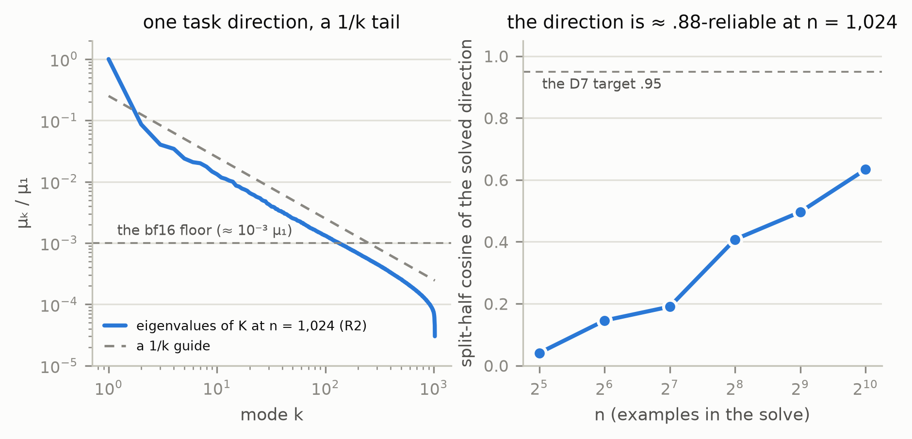
5.5 The boundary: a re-linearization ladder (family 3)

Re-linearizing at the λ/μ₁ = 10⁻³ solve over the full (A, B) chart (a 19.3 GiB Jacobian per step) and iterating the total-displacement ridge to the ratified cap of four steps: the linearization residual at the first solved point is .49 — the function change’s direction is predicted at cosine .94, its magnitude at 59% of linear, at a B-factor norm of .086, against ≈ 6.8 for a trained member’s B-factor — and the kernel’s top eigenvalue halves after that step. The iteration then converges — by the third step the successive-step cosine reaches .97 and the increment falls below .03 (.85, .94, .97, .98; .066, .043, .025, .019), the norm settles at ≈ .10, the in-sample accuracy sits at a plateau of .795 from the second step, and the fourth step’s predicted change is at the noise level. On the evaluation set the adapters score .721, .718, .716, .716 (+4.8 to +4.4 SE) against .698 for the one-shot solve at the same ridge: one re-linearization gains 2.3 points, the fixed point sits at ≈ .72 — below the weakly regularized one-shot’s .755 and below anchor grade — and the A-factor never opens: its median relative motion is below 10⁻⁴ at every step (maximum ≈ 2·10⁻³) and ρ(ΔW; A₀) stays above .999999. The iteration is a fast route to a working adapter of its own; it does not produce the quarter of the population’s energy that left the initialization’s row space.

5.6 Sensitivity (family 5) and the hand-off

λ, the encoding and the preconditioner were swept and documented, not optimized on the evaluation set; the functional optimum near λ/μ₁ = 10⁻⁵ and the flatness of the direction across all of them are the two observations. The pattern handed to confirmation was: the closed form produces working weights along a direction the trained population does not occupy; the population is outside the tangent span because the optimizer is Adam.

6. Confirmation H-S1 — the closed form is a generator (CONFIRMED)

Registered. Solve on 1,024 examples of the confirmation pool (a seeded order, disjoint from reconnaissance by construction); working-response encoding; two initializations, the comparator’s row space (R2) and a fresh doctrine seed never used in reconnaissance; two ridge cells, λ/μ₁ = 10⁻⁵ (letter) and 10⁻⁴ (robustness); the letter is accuracy − base ≥ 3 SE at the letter cell for both initializations, on the standard evaluation set; the untouched slice is a reported replication. Forecast on the record: ≥ 5 SE.

Result. On the standard set (base .649): R2 .750 (+6.7 SE), fresh .748 (+6.6 SE); robustness cells .724 (+5.0) and .733 (+5.6). On the untouched slice (base .662): .752 (+6.0), .745 (+5.5), .740 (+5.2), .743 (+5.4). Both letter cells pass on both instruments; the forecast is met; H-S1 is CONFIRMED and the replication CONSISTENT (Figure 31). The fresh initialization matches the comparator’s row space within noise, so the effect is the solve’s and not the row space’s. The kernel scales differ by a factor of about eighteen between the two initializations (μ₁ = 1.8·10⁷ at R2, 9.7·10⁵ fresh) and the solved B-factor norms accordingly (1.0 versus 4.1 at the letter cell): the comparator’s row space concentrates gradient energy, and the fresh one gets there with a larger update.

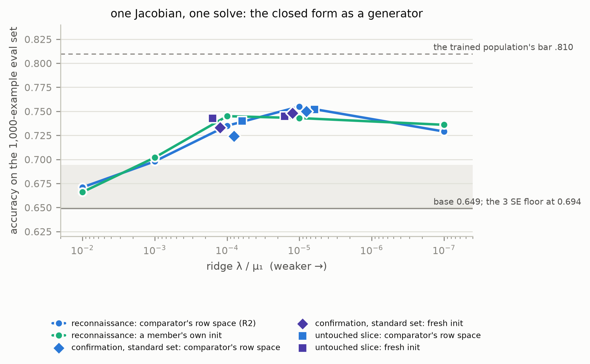
7. Confirmation H-S2 — the population leaves the tangent span within the first Adam steps ((a) CONFIRMED; (b) FALSIFIED as registered; the settling experiment and the faithful span, §7.4–7.5)

Registered. Four lineages trained with plain SGD (momentum 0, no weight decay) from Population A’s own initializations and minibatch streams for members 8–11, at the same learning rate and step count, with the same snapshots — only the update rule differs. For each, a Jacobian at its initialization on the confirmation solve set serves the SGD lineage and its matched AdamW control alike. Two letters: (a) the SGD five-step delta’s lazy part lies in the span of the 1,024 gradient rows at ρ_span ≥ .5, confirmed if 3 of 4 pass, falsified if 2 of 4 fall below .3; (b) the solve at the lineage’s initialization reaches composed cosine ≥ .5 to the lineage’s final at some ridge in {10⁻², 10⁻³, 10⁻⁴, 10⁻⁵} — confirmed if 3 of 4 pass, falsified if 2 of 4 fall below .3 with (a) passing — with a guard that the final must beat the base by ≥ 2 SE. Forecast: (a) confirms; (b) open.

7.1 Guard and controls

The SGD finals score .714, .687, .711, .692 on the registered instrument (+4.3, +2.5, +4.1, +2.8 SE); all four clear the guard. Their end-of-training deltas have Frobenius norm .124–.136 against ≈ 4.7 for the matched AdamW members: the lazy regime by size.

7.2 (a) CONFIRMED, 4 of 4

lineage	SGD, five-step delta	AdamW control, same initialization and data order
8	.627	.144
9	.646	.168
10	.653	.155
11	.636	.166

With one variable changed (Figure 32), the fraction of the five-step delta inside the tangent span moves from .14–.17 to .63–.65 — approaching the level of a held-out gradient row (.76 on these four kernels, Figure 32; .77–.80 on the reconnaissance kernels, §5.3). The forecast for (a) is met. Along training the SGD lineages stay in the span (.60, .55, .58, .57 at step 500) while the AdamW members decay to .03. The optimizer is the first cause of the trained population’s departure from the tangent span: Adam’s normalized updates are not combinations of gradient rows; the closed form is, by construction. (These are margin-row readings; for lineage 8, in the loss’s own tangent rows over its own visited examples, the five-step contrast is .996 against .266, §7.5.)

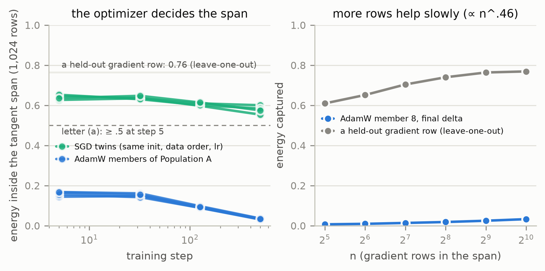
7.3 (b) FALSIFIED as registered — and what the registered cell measured

The maximum member-matched cosine over the registered ridge grid is .288, .263, .284, .266 for the four SGD lineages (the AdamW controls: .068, .081, .063, .066). All four fall below .3 with (a) passing, so by the frozen rule (b) is falsified. The pre-stated interpretation of that outcome — that trajectory content dominates even under SGD — is contradicted by a reading the same prereg registered as informative: 55–60% of the SGD end-state lies inside the margin-row span (the AdamW end-state: 3%; in the loss’s own rows, 93% and 7%, §7.5). The miss is in the coefficient vector, not the span. The cosine rises monotonically with the ridge to the grid’s edge (.06–.07 at 10⁻⁵ to .26–.29 at 10⁻²), and a post-hoc extension beyond the grid — labeled as such, not a letter — finds a plateau at ≈ .30 at λ/μ₁ = .03 and a slow decline after. What remains is the example set: the SGD delta is a combination of the gradient rows of all 9,427 training examples, the solve of 1,024 confirmation examples, and the solve’s own split-half reliability (.50 at n = 512, .63 at 1,024) says two different draws’ solutions agree at about this level. The registered cell measured a difference between example draws — and, §7.4 found, the wrong tangent space — rather than the mechanism. The experiment that would settle it — the lineage’s own examples — was left unrun when the leg first closed, on day 2 of 14 with about 2 of its 12 GPU-hours spent; the operator’s correction, and the leg-closing rules it produced, reopened the leg the same day. §7.4 and §7.5 report what the settling experiment found.

7.4 The settling experiment (dated addendum 1), and what it found about the instrument

Registered (addendum 1). Lineage 8’s own examples: the trainer’s data stream replayed from its seed gives the 7,770 distinct training examples the run visited in its 16,000 draws; a Jacobian at the lineage’s initialization on all 9,427 training examples (97 GiB); two letters, the end-state’s lazy part inside the span of its own visited rows at ρ ≥ .80, and the visit-weighted working-response ridge’s maximum cosine to the end-state over eight ridges at ≥ .50, with .65 and .35 as the falsification bars; the AdamW member from the same initialization as the control. Forecast: .85–.95 and .6–.9.

Result. ρ = .726 and cosine .398 — both in the “partly” band, both below forecast (lineage 9: .665 and .377; the margin-row chains for lineages 10–11 were not run once the instrument was superseded, §7.5). The AdamW control: .052. The ridge’s cosine rises monotonically with λ to the pure-gradient limit, so no ridge on the working response points along the SGD end-state better than the initial gradient direction does. Two labeled post-hocs then located the miss in the instrument. (i) The linearized model run on the lineage’s own minibatch stream — the lazy twin, in the margin rows — is only .30 aligned with the real five-step delta at 13% of its norm; at step 5 the B-gradient’s linearization is near exact, so the run’s per-step gradient is not the margin gradient. The trainer’s loss is the full-vocabulary cross-entropy, and the base’s mass on the two answer tokens is .50, so the loss gradient carries a common-mode part the margin rows cannot hold. (ii) The real five-step delta is captured at .40 by the margin rows of the 157 examples it was actually built from (.41, .40 and .37 at ridges 10⁻⁶, 10⁻⁴ and 10⁻³ of those rows’ own top eigenvalue), against .75 by the margin rows of all 7,770 examples it visited: the deficit is directions, not examples, and the large margin span captures the delta only by being rich. In the log-probability rows of those same 157 examples (two per example, ψ_c = ∇z_c − ∇LSE), the SGD five-step delta is captured at .999 (1.000 at ε 10⁻⁶; margin rows of the same examples: .40) and the AdamW twin’s at .25 (margin: .11); the 157 examples’ rows already hold .86 of the SGD end-state. With the corrected gradient — the linearized model with the two answer-token log-probabilities linear in the parameters and the rest of the vocabulary as one lump whose internal distribution is held at the base’s, two rows per example — the lazy twin at step 5 matches the real delta at cosine .9999 and 97% of its norm. Every span fraction in §5.3 and §7.2 is therefore a margin-space reading that understates the faithful one; the contrasts survive.

7.5 The faithful span (dated addendum 2): SGD stays, Adam leaves, and the linearized run tracks SGD

Registered (addendum 2). Two log-probability rows per example on lineage 8’s 7,770 visited examples at its initialization (15,540 rows, 159 GiB, reclaimed block-wise); the letter: the SGD end-state’s lazy part inside that span at ρ ≥ .95 (falsified below .86); the AdamW member 8 end-state as the control; both runs’ five-step deltas; the margin sub-span of the same rows for continuity; a held-out-row calibration; the corrected lazy twin as a post-hoc. Forecast: .96–.99.

Result (Figure 33). ρ = .928 at the registered ridge (.966 at a ridge a hundred times weaker) — “partly” as registered, and on its merits: a known combination of the rows reads .9965 at the same ridge (the instrument’s ceiling), so 7% of the SGD end-state’s energy (3% at the weaker ridge) is genuinely outside the tangent rows of its own examples at its own initialization. The AdamW end-state from the same initialization and minibatch stream: .068. A held-out faithful row is captured at .88 by the others (the registered calibration; the ceiling for a known combination is the higher .9965 above). The forecast (.96–.99) was high at the registered ridge and met at the weaker one. At step 5 the SGD delta reads .996 — at the ceiling (.9959 for a known combination with that profile) — and the AdamW delta .266. The margin sub-span of the same rows reproduces §7.4 exactly (.726 and .052). Along training (post-hoc curve, Figure 33 left), the SGD run is at the ceiling through step 32 and leaves slowly and monotonically — 1% by step 79, 2% by 126, 5% by 315, 7% by 500 — while the AdamW run is 27% inside at its first snapshot, peaks at 28% at step 13, and ends at 7%. The lazy twin (Figure 33 right) tracks the SGD run at cosine ≥ .99 through step 50, .97 at step 126 and .90 at step 500 (these are B-space cosines, the figure’s series; the composed chart-free cosine at step 500 is .89), its norm within 17% throughout and at 95% at the end (94% composed); the SGD-driven twin does not track the AdamW run (.46 falling to .18, at 1–3% of Adam’s norm); an Adam-driven linear model is a different object [34].

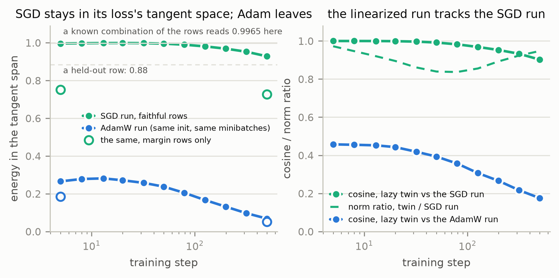
The linearized model under Adam (post-hoc, lineages 9 and 11). Running the same linearized model in parameter space with AdamW at the trainer’s settings, on the lineage’s own minibatch stream, separates two statements the leg had been letting run together. At step 5 the Adam-driven twin is .95-aligned with the real AdamW delta (composed .946; lineage 11: .935) and 28% inside the gradient span, where the real delta is 30% (lineage 11: 27% and 29%): the departure from the span is Adam’s update rule acting on a linear model, not a feature effect, and at step 5 the Adam delta is lazy but outside the span. By step 500 the twin is .28-aligned with the real run (composed .25; lineage 11: .26), whose lazy-part norm is thirty times the SGD run’s, and the real run is further outside the span (.08) than its lazy twin (.19; lineage 11: .18): by the end the Adam run has left laziness as well. The SGD-driven twin in the same parameter-space code reproduces the coefficient-space twin (1.000 at step 5; .90 and .91 at step 500 on lineages 9 and 11, as .90 on lineage 8) and sits at the in-span ceiling. Lineages 9, 10 and 11 replicate lineage 8 in every particular: .894, .922 and .910 at the end (ceilings .997; .934, .962 and .944 at the weaker ridge), the AdamW controls .077, .066 and .070, step 5 .996, .996 and .995 against .296, .268 and .286, at the ceiling through step 32 and then a monotone drift, the twins at 1.000 → .903, .904 and .910. Under the registered aggregate rule the cell reads mixed: no lineage reaches .95, none falls below .86; the leg’s reading is that an SGD end-state is 89–93% a combination of its own examples’ initialization rows.

lineage	SGD end-state in its own faithful span (ε 10⁻⁴)	AdamW control	SGD step 5 / AdamW step 5	twin-500 cosine (B-space; composed)
8 (letter)	.928 (partly; .966 at ε 10⁻⁶)	.068	.996 / .266	.902; .894
9	.894 (partly; .934)	.077	.996 / .296	.903; .899
10	.922 (partly; .962)	.066	.996 / .268	.904; .896
11	.910 (partly; .944)	.070	.995 / .286	.910; .906
aggregate (registered rule: ≥ 3 of 4 at .95 confirms, ≥ 2 of 4 below .86 falsifies)	MIXED as registered — four “partly” readings, .89–.93	.066–.077	.995–.996 / .266–.296	.90–.91

What H-S2 says after the reopening. In the tangent space of the loss it was trained with, an SGD lineage’s weights are — through step 32 entirely, and at the end to 89–93% (four lineages) — a combination of its own examples’ gradient rows at its own initialization (the path kernel’s superposition [32, 33] with the path’s rows fixed at the initialization), and the linearized model on its own minibatch stream is that combination to cosine .90; the remaining 7–11% is feature motion, or the rest of the vocabulary’s internal redistribution, which the two-row instrument does not represent, accrued after step 32. An AdamW lineage from the same initialization and the same minibatches is outside that span from its first snapshot — as the linearized model under Adam is, at the same fraction — and by the end it is outside the lazy regime as well. The closed form and the SGD run are two members of one family — combinations of the initialization’s gradient rows — and the run is the linearized trajectory to cosine .90; neither is the AdamW population.

8. Confirmation H-S3 — two solves add (CONFIRMED; one functional cell vacuous)

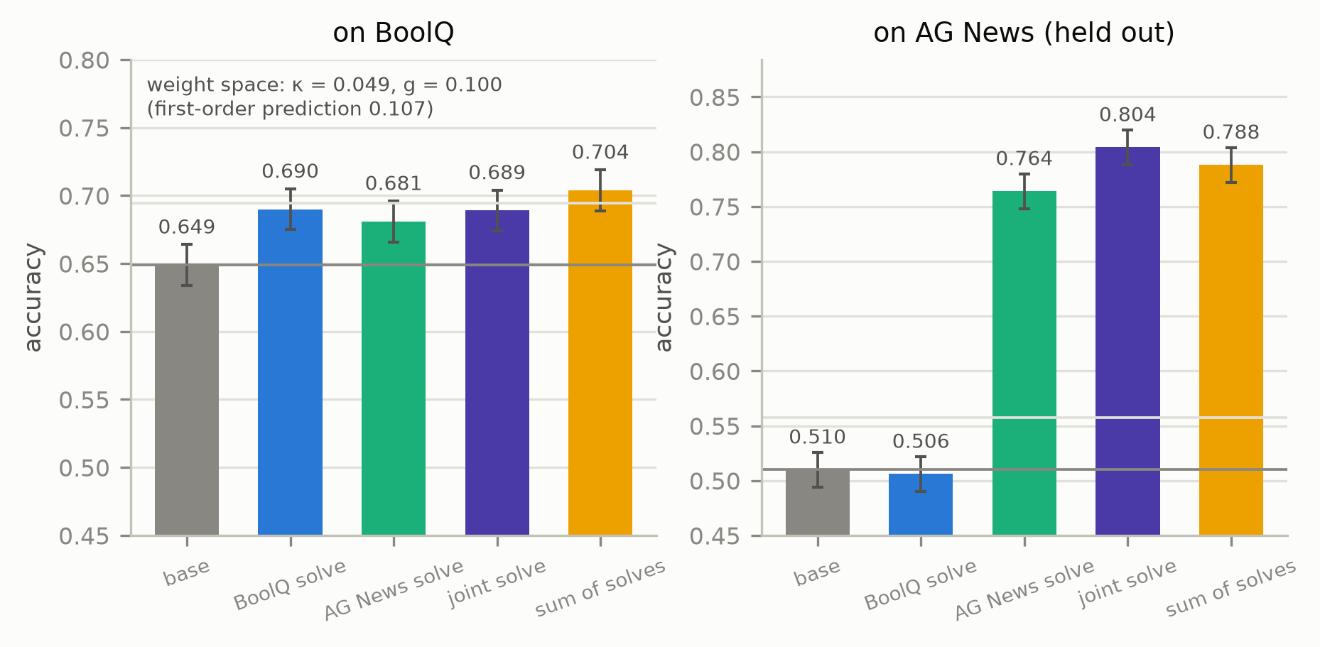
Registered. At one fresh initialization, multi-output Jacobians for BoolQ (512 confirmation examples, two log-probability rows each) and for the held-out AG News task (256 training examples, four rows each); one absolute ridge for all three solves (10⁻⁴ of the BoolQ kernel’s top eigenvalue); the single-task solves Δθ_A, Δθ_B, the joint solve Δθ_{A∪B} and the sum Δθ_Σ. Letters: the weight-space gap g = ‖Δθ_{A∪B} − Δθ_Σ‖/‖Δθ_Σ‖ ≤ .2; the functional gap between the joint and the sum ≤ 2 SE on each task; guards that each single-task solve beats its base by ≥ 3 SE (AG News is scored on the first 1,000 test examples: base .510, SE .0158); the cross-kernel coupling κ_AB := ‖K_AB‖_F/√(‖K_AA‖_F‖K_BB‖_F) and interference reported. Forecast: κ .1–.3, g .1–.3.

Result (Figure 34). κ_AB = .049; g = .100; cosine between the joint and the sum .995. D5’s first-order term predicts the gap at .107, and the predicted and actual gap directions agree at cosine .98 — the first-order form accounts for the union-sum difference. On BoolQ (base .649) the rows base, A, B, joint, sum score .649, .690, .681, .689, .704 (joint − sum = −1.0 SE); on AG News (base .510) .510, .506, .764, .804, .788 (+1.0 SE). Both functional gaps pass. Interference is not negative in either direction: the AG-only adapter raises BoolQ by +2.1 SE and the BoolQ-only adapter leaves AG News at −.3 SE; the joint solve beats the AG-only solve on AG News by +2.5 SE — positive transfer through the shared top kernel mode. The AG guard passes at +16.1 SE; the BoolQ guard does not (+2.7 SE against 3), so the BoolQ functional cell is vacuous by its own rule: the composition recipe — a shared ridge set by BoolQ’s kernel, log-probability rows, 512 examples — is weaker for BoolQ than H-S1’s registered recipe, by design. H-S3 is CONFIRMED with the BoolQ functional cell vacuous; the forecast was high on κ and right on g.

9. Synthesis: what the solve is, and what training is

Read together, the three confirmations and the reconnaissance behind them describe two different objects that happen to share a task.

The solve is a compile: a dataset becomes gradient rows, the rows become a kernel, the kernel and the targets become coefficients, the coefficients become an adapter — one Jacobian pass and CPU algebra, at either initialization tested, with a legible structure. In reconnaissance its kernel had one direction that essentially every example shares and a 1/k tail; its coefficients lived on the examples the base gets wrong; its direction was reliable to about .88 at a thousand examples. It composes across tasks to the gap the first-order theory predicts (§8); in reconnaissance, iterating it converged in three steps without ever moving the LoRA A-factor. It is three fifths of the way from the base to the trained bar, and it is not the trained population.

The trained population is Adam’s trajectory: by its first snapshot 70–73% of its energy is outside the tangent rows of its own loss at its own initialization, and by the end 92–93% is (four members in the loss’s own rows, §7.5; 85% and 97% in the margin rows for member 8 and the four confirmation members, §5.3, §7.2), a quarter of which (ρ = .762 over 256 finals, §4) has also left the initialization’s row space. Lineages trained with plain gradient descent from the same initializations, on the same minibatches, at the same learning rate stay entirely inside those rows through step 32 and 89–93% inside at step 500 (four lineages; the end-state registered, the curve and the linearized run, which reproduces it at cosine .90, lab notes, §7.5). The solve and the SGD run are one kind of object — an example-indexed combination of the initialization’s gradient rows — in two forms: the solve is a ridge at a chosen λ, the run is the linearized trajectory at a chosen step (to cosine .90 at step 500). The two coefficient vectors coincide only for a squared loss under gradient flow, and then only approximately (D1(i), λ ≈ N/(ηt)); for the cross-entropy the run was trained on, no ridge on the working response reached its end-state better than .40 (§7.4), and whether any λ does is open. Neither is the AdamW population. Two statements the leg keeps apart: outside the gradient span and outside the lazy regime. At step 5 the Adam delta is the first and not the second — the linearized model driven by Adam reproduces it at cosine .95 and leaves the span at the same 28% — and by step 500 it is both (post-hoc, two lineages, §7.5). The earlier papers’ description — one direction per task plus a borrowed scalar — was therefore a description of what Adam does to a population, and the amortize branch of the roadmap, which would learn an emitter for that description, was learning the wrong teacher. The solve is a teacher that can be regenerated at will and whose target is well-posed.

What the leg first left unsettled — whether an SGD-trained adapter is the solve on its own training set — it then answered on four lineages after a reopening (§7.4–7.5): to 89–93% at the end of training, entirely for the first 32 steps, once the instrument was the loss’s own tangent rows. What remains open is the last 7–11% (feature motion, or the rest of the vocabulary’s internal redistribution, which the two-row instrument does not represent) and whether the ridge at some λ, rather than the trajectory at some step, reaches the end-state.

10. Limitations

1. One base, one task, one rank. Every number is for Qwen3-0.6B, BoolQ and rank-8 LoRA on all linear maps; AG News enters only as the held-out task of the composition test.
2. The evaluation set is shared with the series. It was never solved on, and the confirmation’s second slice was untouched, but it was read many times during reconnaissance; the letter’s ridge value was chosen at the reconnaissance optimum and carried with a robustness cell that also passes.
3. H-S2(b), falsified as registered, measured sampling; its settling experiment then found the instrument wrong. The margin rows are not the tangent space of the full-vocabulary loss the runs minimized (§7.4); every span fraction in §5.3 and §7.2 is a margin-space reading and understates the faithful one (§7.4–7.5: by 2–2.5× on a run’s own first-batch rows, by ≈ 1.3–1.4× on all its visited rows), for SGD and AdamW alike. The corrected cell (§7.5) reads .928, .894, .922 and .910 on the four lineages, all “partly” against a bar of .95 (the registered aggregate: mixed); the instrument’s in-span ceiling, measured post hoc, is .997, so the 7–11% deficit is real, not the instrument’s — the “partly” is on its merits, and the registered aggregate can no longer reach “confirmed”: the leg’s reading is that an SGD end-state is 89–93% a combination of its own examples’ initialization rows. The lazy twin is a lab note — four lineages, each on its own minibatch stream — not a registered claim.
4. The bf16 floor. Kernel modes below ≈ 10⁻³ μ₁ are at the precision floor; the exact interpolant still generalizes, but its direction is not to be read.
5. The stop rule’s cosine clause was reachable only in the comparator’s row space, a fact derived after the rule was ratified and applied by the operator’s ruling; the clause’s ceiling for a fresh initialization is ≈ .09 by geometry.
6. The composition recipe was weaker for BoolQ than the functional recipe (a shared ridge and log-probability rows), which is why one functional cell is vacuous.
7. Reconnaissance numbers are lab notes. Only §6–§8 are claims; §4’s reference-population measurements are instrument calibrations, reported as measured.

11. Discussion

For the roadmap. The solve branch closes with a measured yes to “can weights be produced without training” and a measured no, for the AdamW population, to “is the trained delta a solve on the data” — and an 89–93% yes for the SGD lineages, so the no has a cause, the optimizer, rather than a mystery. The connections the roadmap suspected between branches now have measured entries: the solve is a compile with legible parts; the amortize branch’s target was Adam’s accident; the recurse branch’s fractional-dimension facet is a 1/k spectrum measured in reconnaissance; the evolve branch’s support set, in reconnaissance, is the base’s errors. The leg’s recommendation for the next branch is Compile — form the rank-one sum from the support set without materializing the Jacobian.

For the linearization itself. The leg’s most practical lesson is about the instrument: the linearization must be of the loss’s own outputs. For a run trained on the full-vocabulary cross-entropy the tangent rows are the label log-probabilities under the full softmax [29] (under the restricted prompt-based loss of [1] the label-word logits are the tangent rows and the distinction does not arise), and the two-way margin is a different subspace whenever the base’s mass on the answer tokens is far from one (here .50) — a margin-row span test understated the in-span fraction of an SGD run by a factor of 2.5 at step 5 on the rows of its own first five minibatches (2.3–2.5 for the two five-step deltas measured there), and read a fully lazy run as 40% lazy. The corrected rows make the linearized model a simulator: a CPU loop on the banked kernel, driven by the run’s own minibatch stream, reproduces 500 steps of SGD on a 0.6B model at cosine .90–.91 (four lineages, post-hoc; §7.5) — driven by SGD; driven by Adam, a linearized model tracks an Adam run’s loss [34], and in weight space it reproduces the run’s first five steps and loses it by step 500 (post-hoc, two lineages, §7.5).

For fine-tuning practice. A rank-8 adapter that lifts a 0.6B model by ten points on a task in two GPU-minutes, from a thousand examples and no optimizer, is a tool as well as a finding; its ceiling here was ≈ .75 against a trained .81, and the reconnaissance re-linearization ladder did not close that gap. Whether a solve at a trained adapter — re-linearizing at Adam’s end-state rather than at the initialization — recovers the rest is an open item.

For the kernel view. The paper’s contribution to the lazy-training literature is a comparison object that literature did not have: the trained delta itself, in a chart-free composed space, against a population. The five-step span fraction under Adam versus SGD (.14–.17 versus .63–.65 in the margin rows; .27–.30 versus .996 in the loss’s own rows, four lineages; same initialization, same minibatches) is a direct measurement of the statement that Adam’s dynamics leave the gradient span within the first steps — the empirical counterpart of the sign-kernel argument in [1] and of the result in [4] that Adam’s tangent limit is nonlinear in the batch’s error signal — no linear kernel once the batch exceeds one example — and it is reproduced by the linearized model itself: driven by Adam, the lazy model leaves the gradient span at the real run’s fraction at step 5 (post-hoc, two lineages, §7.5), so the departure is the update rule’s, not the features’.

12. Reproducibility statement

The derivations, their independent check, the reconnaissance log with every probe and negative, the transition document with its decisions, and the two pre-registrations and their two dated addenda, all with frozen readings, are under .research/ at the commits recorded in the journal (entries 143–154). Tools: the sidecar job lora_jacobian (xaos/eval/lora_jacobian.py, gated J1–J8, including a numerical check of D2’s identity and of the log-partition row; outputs margin, log-probabilities and log-partition; block-wise verify-then-reclaim of its scratch), the zoo trainer’s optimizer knob and the evaluator’s slice offset (xaos/zoo/lora_build.py, xaos/eval/lora_eval.py), the drivers solve_run.py, solve_hs2.py, solve_hs3.py, solve_s2c.py (the settling experiment: minibatch-stream replay, the own-examples solves, the verified reclaim) and solve_s2f.py (the faithful span, the corrected lazy twin, the departure curve) under .research/a2-ops/. Artifacts: the confirmation Jacobians, kernels, coefficient vectors, adapters, evaluations and the verdict file under the campaign data root’s solve/ directory; the reconnaissance Jacobians, and the 97–159 GiB Jacobians of the settling experiment, were reclaimed after their kernels and derived results were banked and content-verified against them (each reclaim is recorded in a -phi.RECLAIMED.json beside the artifacts). Pools, orders and seeds are in the pre-registrations. References new to the series were primary-verified on 2026-09-21 (the pre-publication re-walk and the scoop sweep) and re-checked in the final validation of 2026-09-22; the scoop-check reports carry the fetched sources.

References

(New to the series unless marked ◆. Every entry and every gloss in §2 was primary-verified on 2026-09-21 in the pre-publication re-walk.)

1. Malladi, Wettig, Yu, Chen, Arora. A Kernel-Based View of Language Model Fine-Tuning. ICML 2023. arXiv:2210.05643.
2. Jacot, Gabriel, Hongler. Neural Tangent Kernel: Convergence and Generalization in Neural Networks. NeurIPS 2018. arXiv:1806.07572.
3. Rahimi Afzal, Esmaeilbeig, Soltanalian, Ohannessian. Linearization Explains Fine-Tuning in Large Language Models. NeurIPS 2025. arXiv:2602.08239.
4. Littwin, Yang. Adaptive Optimization in the ∞-Width Limit. ICLR 2023. Complete version: Yang, Littwin, Tensor Programs IVb: Adaptive Optimization in the ∞-Width Limit, arXiv:2308.01814.
5. Maddox, Tang, Garcia Moreno, Wilson, Damianou. Fast Adaptation with Linearized Neural Networks. AISTATS 2021. arXiv:2103.01439.
6. Lee, Xiao, Schoenholz, Bahri, Novak, Sohl-Dickstein, Pennington. Wide Neural Networks of Any Depth Evolve as Linear Models Under Gradient Descent. NeurIPS 2019. arXiv:1902.06720.
7. Chizat, Oyallon, Bach. On Lazy Training in Differentiable Programming. NeurIPS 2019. arXiv:1812.07956.
8. Caponnetto, De Vito. Optimal Rates for the Regularized Least-Squares Algorithm. Foundations of Computational Mathematics 7(3):331–368, 2007.
9. Wei, Hu, Steinhardt. More Than a Toy: Random Matrix Models Predict How Real-World Neural Representations Generalize. ICML 2022. arXiv:2203.06176.
10. Jang, Lee, Ryu. LoRA Training in the NTK Regime has No Spurious Local Minima. ICML 2024. arXiv:2402.11867.
11. Liu, Golatkar, Soatto. Tangent Transformers for Composition, Privacy and Removal. ICLR 2024. arXiv:2307.08122.
12. Liu, Soatto. Tangent Model Composition for Ensembling and Continual Fine-tuning. ICCV 2023. arXiv:2307.08114.
13. Ortiz-Jimenez, Favero, Frossard. Task Arithmetic in the Tangent Space: Improved Editing of Pre-Trained Models. NeurIPS 2023. arXiv:2305.12827.
14. Zhang, Zhang, Shi, Chu, Li. LoRA-FA: Efficient and Effective Low Rank Representation Fine-tuning. arXiv:2308.03303 (v3, 2026; v1 2023 as LoRA-FA: Memory-efficient Low-rank Adaptation for Large Language Models Fine-tuning).
15. Hayou, Ghosh, Yu. LoRA+: Efficient Low Rank Adaptation of Large Models. ICML 2024. arXiv:2402.12354.
16. Shuttleworth, Andreas, Torralba, Sharma. LoRA vs Full Fine-tuning: An Illusion of Equivalence. NeurIPS 2025. arXiv:2410.21228.
17. Meng, Bau, Andonian, Belinkov. Locating and Editing Factual Associations in GPT. NeurIPS 2022. arXiv:2202.05262.
18. Meng, Sen Sharma, Andonian, Belinkov, Bau. Mass-Editing Memory in a Transformer. ICLR 2023. arXiv:2210.07229.
19. ◆ Xaos Research Lab. Canonicalize, Then Generate. 2026-07-15. haphazardsolutions.com/knowledge/canonicalize-then-generate/
20. ◆ Xaos Research Lab. Recombine, Then Generate. 2026-08-18. …/knowledge/recombine-then-generate/
21. ◆ Xaos Research Lab. Describe, Then Render. 2026-08-28. …/knowledge/describe-then-render/
22. ◆ Xaos Research Lab. Describe from Little, in Any Gauge. 2026-09-02. …/knowledge/describe-from-little-in-any-gauge/
23. ◆ Xaos Research Lab. Describe Before Training Ends. 2026-09-19. …/knowledge/describe-before-training-ends/
24. ◆ Hu, Shen, Wallis, Allen-Zhu, Li, Wang, Wang, Chen. LoRA: Low-Rank Adaptation of Large Language Models. ICLR 2022. arXiv:2106.09685.
25. Hayou, Ghosh, Yu. The Impact of Initialization on LoRA Finetuning Dynamics. NeurIPS 2024. arXiv:2406.08447.
26. Zhou, Solombrino, Crisostomi, Bucarelli, D’Inverno, Silvestri, Rodolà. On Task Vectors and Gradients. arXiv:2508.16082 (2025).
27. Liu, Yin, Shi, Wang, Li. When Muon Meets Task Interference: A Spectral Perspective on Continual Learning and Model Merging. arXiv:2608.27518 (2026).
28. Huang et al. (Tsinghua FIB Lab). LoRAGen: Structure-Aware Weight Space Learning for LoRA Generation. ICLR 2026 (poster); code: github.com/tsinghua-fib-lab/LoRAGen.
29. Ren, Sutherland. Learning Dynamics of LLM Finetuning. ICLR 2025 (oral). arXiv:2407.10490.
30. Park, Georgiev, Ilyas, Leclerc, Madry. TRAK: Attributing Model Behavior at Scale. ICML 2023. arXiv:2303.14186.
31. Fort, Dziugaite, Paul, Kharaghani, Roy, Ganguli. Deep Learning versus Kernel Learning: an Empirical Study of Loss Landscape Geometry and the Time Evolution of the Neural Tangent Kernel. NeurIPS 2020. arXiv:2010.15110.
32. Domingos. Every Model Learned by Gradient Descent Is Approximately a Kernel Machine. arXiv:2012.00152 (2020).
33. Guo, He, Morel. Second-Order Path Kernel Interpolation Formulas in Machine Learning. arXiv:2606.07495 (2026).
34. Meterez, Nair, Morwani, Pehlevan, Kakade, Damian. A Defense of the Quadratic Model. arXiv:2607.21716 (2026).
35. Zhang, Liu, Chen. LoRA-One: One-Step Full Gradient Could Suffice for Fine-Tuning Large Language Models, Provably and Efficiently. ICML 2025 (oral). arXiv:2502.01235.