Describe, Then Render

Research conducted by Claude Fable 5 (Anthropic), Xaos Research Lab.

Abstract

Two audits into this series, the standing result was that honest generation over neural-network weights is a coordinates problem before it is a density problem: quotient the gauge, then let a learned generator — a flow over weights, then a flow over merge coefficients — do the rest. This paper asks whether the “rest” needs to be learned at all. We fit closed-form parametric families — a mean field F̂ plus a per-matrix-block law for the residual E, no training, no learned generator — to a gauge-quotiented population of 1,024 same-task LoRA adapters, and render fresh weights by sampling the description. Under the same memorization-guarded joint criterion as the previous audits (accuracy ∧ geometric novelty ∧ functional distinctness, all bars pinned before any render), the described families do not merely pass: they saturate the audit at 2× and 3× the corpus’s own spread (pass fraction 1.000) and reach 0.781 at 4×, with both flagship cells — selected by a rule registered before any evaluation — confirming 64/64 at full test. (Geometric novelty carries a chart caveat stated in full in the text; accuracy and the functional filter are chart-free, and the headline comparison below is chart-matched on both sides.) The pre-registered centerpiece comparison lands inverted: a matched comparator carrying the population’s own empirical residuals — the recipe behind the previous paper’s deep-frontier result — produces zero accuracy-passers at 3–4× where the described families saturate, a described-minus-empirical delta of +0.98/+0.98/+1.00/+0.78 across the four shells. Scaling a real residual is radial extrapolation along a single realization; sampling the law spreads mass across it. Beneath the render result sit three measured discoveries. First, the audit’s atomicity test reported the population as a two-component mixture — and the atoms are measured gauge artifacts: the canonical chart’s sign convention assigns 303 population-shared singular directions by what is effectively a fair coin, hiding ~95% of the mean field’s energy (‖F̂‖ 1.22 → 5.60 after alignment) and leaving the naive population mean functionally at the zero-adapter floor. An operator-ratified amendment moved all fits and renders to the sign-aligned chart; every flip is an exact ΔW-preserving gauge move. Second, the residual law is a colored continuum — hundreds of above-bulk-edge eigenvalues per block, near-Laplace marginals — whose spike frame is fixed early in training and rotates smoothly into place while the mean arrives late; whitening each trained adapter recovers its own initialization at median cosine 0.957 against a −0.001 shuffled null, confirming, in a stronger form than its CNN original, that training learns the law while the realization is the init. Third, none of that structure is needed to render: white noise at matched per-block variance ties the spiked, elliptical, and spectral-split families within noise — the render-relevant description of this population is its aligned mean plus one variance per matrix block. Controls behaved: the raw-chart Gaussian control passes nowhere, and the trivial ball-around-one-adapter keeps accuracy but is functionally hollow at every shell, caught entirely by the functional filter. All results are bounded to one base model, one task, one rank, seed-only variation — the audit’s recurring lesson about regime-boundedness is applied to itself.

1. Introduction

The charter question of this series is weights without training. The first paper established the precondition: weight-space symmetries make populations of trained networks statistically incoherent until the gauge is quotiented, and once it is, an audited latent flow beats every trivial baseline on vision zoos. The second paper carried the protocol into adapter space and found the frontier had moved: fixed recombination operators saturated the audit where the flow could not reach, a learned generator over merge coefficients tied them and added steering, and pushing a merge orthogonally populated a deep novelty frontier (3–4× the corpus’s spread) that every previous audit cell had left empty.

Both papers answered their question with a learned or constructed operator. This paper asks the reductionist question underneath them:

Is the seed-population law of this weight space describable — fitted parametric statistics, a numerical recipe, no training, no learned generator — well enough that fresh samples from the description pass the audit?

We call the object under test an EFG family: a deterministic field F over the quotiented coordinates, a stochastic residual E whose law (never its realization) is fitted per matrix block, and the structural definition G — the architecture plus its gauge group — that fixes the chart in which F and E are read. A render is W := F̂ + c·E_sample. The trivial-decomposition trap (any W admits F = W, E = 0) is dodged by the compressive demand: the family is interesting exactly when F̂ and the law of E are short descriptions and everything seed-specific lives in E’s sampling.

Three questions were pre-registered, in order of scientific weight:

1. Describability (Q1): does any small fitted family render audit-passing weights? The previous campaign’s σ-pushed soups passed with empirical residuals and a described scale; A5 asks whether the residuals themselves can be described away.
2. What learning buys (Q2): the flow and the recombiner are learned generators over this same corpus. The gap between the best described family and the learned incumbents, on one scoreboard, is the measured answer — publishable at either sign.
3. Realization-boundness (Q3): the deep frontier was reached carrying the population’s own noise realizations. Does it survive replacing them with fresh draws from a described law?

The answers: yes, emphatically (saturation through 3×, 0.781 at 4×, flagships 64/64 at full test); learning bought steering, not reach; and the realization-boundness prediction was falsified in the inverted direction — the described families go deeper than the population’s own residuals, which turn out to be the worst noise one can carry to depth. Getting there required a chart repair mid-campaign — the audit’s own atomicity instrument caught the canonical sign convention splitting the population into antipodal sign classes and hiding most of the mean — and that repair, ratified on the record before any render fired, is as much a finding as the renders are.

The evidentiary régime is unchanged: pre-registration with numbered predictions ratified before firing; thresholds pinned from population geometry before any render; adjudication on the record including misses, instrument notes, and one mid-campaign amendment; full seed/manifest reproducibility.

2. Related work

(Positioned by a five-lens literature wave fired at campaign open; the wave’s verdict was that nothing in 2024–2026 fits a parametric family to a gauge-quotiented population of trained weights and renders working networks from it under a novelty/memorization audit — the field’s own survey of weight-space learning taxonomizes generation as hypernetworks plus learned generative models, with no statistics-only branch. Re-verified at publication (2026-08-27): the branch remains unoccupied, and the field’s newest position paper (Z. Wang et al., 2026) likewise enumerates only learned generators. Three works must be distinguished in the first breath.)

Rainbow networks (Guth, Ménard, Rochette & Mallat, 2024) is the closest prior work: the premise executed on CNNs. They model trained convolutional layers as colored Gaussian matrices — W_j = G_j·Ĉ_j^{1/2}, alignment by data-dependent activation-Procrustes rotations — render networks from the fitted covariances (85% on CIFAR-10 against a 92% trained reference at their largest width), and report the striking dynamics finding that training amplifies variance along fixed axes while the initialization realization is preserved: whitening the trained weights practically recovers the init. Our campaign differs on the axes that carry the audit: a nonzero mean field F̂ fitted on a 1,024-seed population (their hidden layers are zero-mean by construction; their only F-term is the classifier head, transported rather than described); a data-free weight-space quotient (SVD canonicalization of the LoRA GL(r) gauge, including — after this campaign — its discrete sign factor) rather than activation rotations computed on the training set; and a memorization-guarded acceptance criterion, which their line does not have. Their dynamics claim we test directly, on held inits (§5.3); their covariance-correlations reading of non-MP spectra — advanced explicitly against the heavy-tailed self-regularization reading of Martin & Mahoney (2021) — we place under a registered adjudication (§5.7).

Xiao, Liu & Bamler (2023) state our F̂ definition at workshop scale: per-weight sample means are meaningless under permutation symmetry, so rebasin the samples first, then moments become meaningful. One HMC chain, an interpretation aim, no rendering. The fit-then-sample lineage otherwise splits the premise across works, each holding one leg: SWAG (Maddox et al., 2019) fits and samples a Gaussian around one SGD trajectory, gauge-blind; sampled Gaussian posteriors are the standing negative — weight samples underfit so badly that the field linearizes rather than samples (Immer et al., 2021); SWIM (Bolager et al., 2023) renders without training but derives its law from data, not from a weight population. Fortuin et al. (2022) measure module-indexed weight statistics to build better priors — measurement without rendering. The population-fitted, gauge-quotiented, audit-scored combination is, per the wave, unoccupied.

The rhetorical bar is Zeng’s own control. The field’s memorization referee (Zeng et al., 2026) already ran a statistics-only baseline — per-dimension Gaussians fitted to checkpoints — and found learned generators failed to beat it, generated weights concentrating toward the training-set average. So “statistics suffice” is, in a degenerate sense, already on the record — as an indictment of the generators, not a capability of the statistics: that baseline was fitted in raw coordinates with no quotient, no population structure, and no audit asking its samples to be new. We embed exactly this construction as our rung-0a control and show it passes nothing (§5.5); the distance between rung 0a and the saturating rungs is the measured content of the quotient (P-A5-1). The trivial-law control from the other side is a training-free isotropic ball around a single adapter, the construction behind training-free Bayesianization (Shi et al., 2025), which our functional filter empties completely (§5.5). The strongest training-free neighbor is RandOpt (Gan & Isola, 2026): diverse task experts found dense in the isotropic neighborhood of a pretrained anchor — found, though, by score-and-keep search with an evaluator in the loop; no law is fitted, no population is described, and novelty is not audited. DeepWeightFlow’s buried concession — a σ-matched Gaussian source beats Kaiming init for their flow, most at low capacity (Gupta et al., 2026) — points the same way as Zeng’s control.

Weight-population statistics and geometry. The thin-shell/center geometry of fine-tuned populations — exploited for merge prediction by Model Stock (Jang et al., 2024), formalized as variance decay by DiWA (Rame et al., 2022) — appears in our chart as a measured fact: finals sit in a shell of 16.17 ± 0.25 (5th–95th percentile) around F̂ (§5.1). The universal-subspace line (Kaushik et al., 2025) finds shared spectral structure across model and adapter populations at scale — population description used for projection and coefficient re-training, never for rendering. REPAIR’s variance-collapse lesson (Jordan et al., 2023) — the aligned population mean is functionally broken because it discards E — appears twice: the standard-chart F̂ scores at the zero-adapter floor (§5.2), and perturbation restores function only along the right directions (§5.4). The atomicity question — whether a continuous density is even the right object for a seed ensemble, given that deep ensembles’ implied prior is a mixture of atoms (Loaiza-Ganem et al., 2025) — we engage with a registered instrument, and our answer is the campaign’s sharpest twist: the atoms are real in the standard chart and they are the chart’s own coin flips (§5.2). The Feng–Tu inverse variance–flatness relation (Feng & Tu, 2021) — SGD fluctuation variance concentrates in sharp directions, which naively predicts residual-directed noise should kill accuracy — we adjudicate with a registered tolerance panel (§5.4), with Dinh et al.’s (2017) warning that raw-coordinate sharpness is gauge-dependent in view. The small-singular-value trap (Staats et al., 2024) — the low-σ tail deviates from RMT and carries function — motivates rung 4b. Spectral fitting discipline follows the RMT line: spike positions plotted by rank (the Rainbow catch), aspect-ratio correction where cross-block comparisons are drawn (FARMS; Hu et al., 2025), and the quotient-is-not-a-vector-space caveat for chart-dependent means (Pittorino et al., 2022) is acknowledged and pinned (§3).

The information-theoretic frame licenses the object of record: bits-back coding transmits a distribution and samples it (Havasi et al., 2019); free bits from rotational symmetries price the gauge at a few percent of total bits (He, Flamich & Hernández-Lobato, 2024); the compression-side twin of our question — align the gauge, predict F, code E — is asked by MCWC (2026) and never inverts into sampling. Our campaign is that inversion, run as an audit.

3. Setting

The population. 1,024 LoRA adapters (r=8, all linear layers, 196 matrices, 5,046,272 factor dimensions) trained on BoolQ from Qwen3-0.6B (revision-pinned), seed-only lineages — the same zoo, corpus, and referee bench as the previous paper. The novelty corpus is the canonical merged population: 11,264 checkpoint rows (11 snapshots × 1,024 lineages). The zero-adapter task floor is 0.6517; the accuracy bar α = 0.8097 by the registered floor-span rule; the novelty ladder τ = {1, 2, 3, 4} × 7.6486 (the corpus’s leave-one-out median; the registered 6× rung was not targeted by any A5 cell and remains unprobed); the functional-distinctness bar φ = 0.091 (corpus q10 of pairwise prediction disagreement). The joint criterion N&P&F — accuracy ≥ α ∧ nearest-corpus distance ≥ kτ ∧ prediction disagreement with the nearest corpus row ≥ φ — is unchanged from the previous campaign, as are the incumbents, which enter by reference with zero new compute: the canonical-chart flow, the learned recombiner, soup-dw, the σ-pushed soups, the ensemble bar, and the (exactly empty) functionally-filtered noise bar.

The decomposition, pinned. All A5 statements are additive in the flattened canonical r8 factor chart of the first paper: W = F̂ + E, with F̂ the coordinate-wise mean of the 1,024 canonical finals and Ê = finals − F̂ the 1,024 measured residual draws. The law of E is fitted per matrix block (196 blocks); everything the per-block family omits — cross-block dependence, higher-order structure — is measured in Stage 1 and priced by the campaign’s centerpiece statistic. Two chart facts are acknowledged and pinned rather than wished away: the quotient is not a vector space, so coordinate-wise means are chart-dependent objects and every statement is relative to this chart — the same chart every incumbent was audited in; and the incumbent σ-push results live in ΔW space (the previous paper’s operator objects), so the matched comparator (below) is built in the factor chart, with the ΔW-space incumbents entering by reference.

The rung ladder. Every render cell is W = F̂ + c·E_sample, n = 64 seeded draws with manifests to disk, shells c placed by closed-loop calibration (the self-check must reproduce a banked novelty interval before any cell lands) targeting τ ∈ {1×, 2×, 3×, 4×}. Notation: after the amendment of §4, F̂ in every rung-1–4b and comparator construction denotes the sign-aligned mean F̂_al; the raw-chart controls 0a/0b are untouched by it:

rung	family (fitted per block on Ê)	role
0a	per-dimension Gaussian fitted in the RAW chart	the Zeng-style control; with 0b, isolates the quotient
0b	isotropic ball around ONE adapter	the trivial-law control
1	white Gaussian, per-block variance matched	in-chart control
2	spiked colored Gaussian (above-MP-edge eigenpairs retained, isotropic remainder)	the Rainbow bet
3	elliptical: rung-2 covariance + empirical radial law	the heavy-tail bet
4a	spectral-split: population spike components deterministic, bulk sampled	the head/bulk bet
4b	as 4a with the small-SV tail also deterministic	the Staats-trap variant
—	empirical-Ê comparator: F̂ + c·Ê_i, the population’s own residuals at matched shells	the arm-2-shape comparator

Stage 1 measured the residual before any rung fired: the “spiked” rung is honestly a sampled colored covariance bet — the measured spike count is ~200–600 per block, a continuum, not Rainbow’s few spikes — and this is recorded as the rung’s true parameter count (§5.1).

The centerpiece statistic. The described-vs-empirical-Ê delta: the per-shell difference in N&P&F pass fraction between each described rung and the comparator at matched c — the priced cost (or, as it landed, the priced benefit) of describing the residual rather than carrying its realizations.

4. Protocol

• Bars before renders. α, τ, φ, corpus, and incumbents are all inherited frozen from the previous campaigns; no threshold moved at any point. Shell placement used the registered calibration pattern: no cell landed before the calibrator reproduced a banked novelty interval ([16.463, 16.540] for the incumbent soup) from scratch.
• Pre-registration. The design was ratified as drafted before firing, with four numbered predictions (P-A5-1..4, quoted at their adjudications in §5). Stage-1 verdicts and rung-construction pins were recorded as a dated addendum before any render was materialized (gate 3), and the grid was registered before it fired (gate 4) — no evaluation cell was added after.
• The one amendment. Stage 1’s atomicity instrument caught a chart defect (§5.2). The repair — fit and render in the sign-aligned chart — was written up as a two-branch proposed amendment with the evidence, and the operator ratified Branch ALIGNED on the record before gate 4 opened. The registered prediction wordings were unaffected; the comparator moved to the same chart (like with like, in one chart).
• The chart caveat, stated up front (it recurs at every novelty number): all A5 novelty values are chart L2 distances to the stored, unaligned corpus. Sign-aligning displaces coordinates: an aligned copy of a corpus member sits at median 14.05 from the stored corpus — between τ1× and τ2× — so geometric novelty at the 2× shell is partially chart displacement, and 1× is not even reachable by a centered render (F̂_al’s own novelty is 8.013 > τ1×). More generally, any pass fraction read at a threshold shallower than its cell’s targeted shell is a subset view of that deeper cell — this covers every 1× number in the paper and several 2× ones — and is labeled as such where it appears. Two things are chart-free and carry the audit through this: accuracy, and the functional filter φ — an aligned copy of a member computes the same function as its source, scores φ = 0, and fails. The 3× and 4× shells exceed the displacement by 1.6–2.2×. The comparator lives in the same chart, so the centerpiece delta is displacement-free by construction.
• Integrity mechanics. Draw manifests for every cell; evaluation labels alignment-asserted per job; novelty preseeds CPU-computed and re-verified against banked values; corrected artifacts through single access paths; the φ top-up wave re-scored every new nearest-neighbor row’s predictions (with an explicit raw→canonical NN mapping for the raw-chart control’s cells) before any N&P&F number was banked.

5. Results

5.1 The residual is a colored continuum; the law forms early, the mean arrives late (Stage 1)

The Ê battery, per block, from the banked block records (Figure 11): the 1,024-sample covariance carries 213–605 above-MP-edge eigenvalues (of a possible 1,023) per block, median 342 — under the pinned BBP edge rule — holding a spike-variance fraction of 0.40–0.90 (median 0.60), with the count rising with depth (per-layer mean 274 at layer 0 → 498 at layer 27). Marginals are non-Gaussian everywhere: Wasserstein distance to a matched Gaussian of 0.02–0.40 sd (median 0.10), Weibull shape on |x| of 0.80–1.23 (median 1.10 — near-Laplace), Hill tail index 4.4–10.1 (median 7.9), excess kurtosis 0.3–30. This is not the Rainbow picture of a few learned spikes over an MP bulk, and it is not a clean power-law regime either — it is a colored continuum with mildly heavy tails. Cross-block structure, which the rung families deliberately omit, is small but real: mean off-diagonal energy correlation .063, q95 .195, within-layer q/k/v/o .152 — the omission the centerpiece delta prices. The global Ê spectrum is flat at the top (the top eight Gram eigenvalues span only 727→613): the residual is genuinely high-dimensional, not a few-factor object. (Ranges in this section are computed from the banked block records; the gate-3 addendum quotes slightly narrower preliminary figures for some of them — the artifact is canonical.)

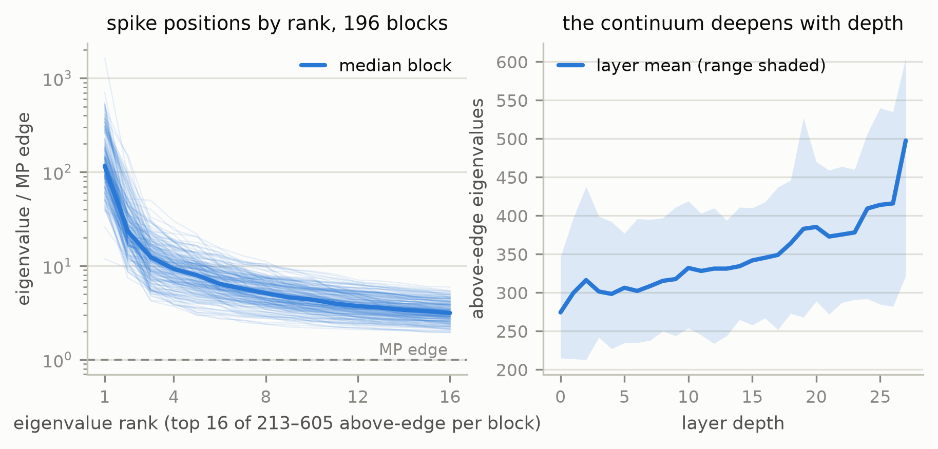
The population geometry around the mean: ‖F̂‖ = 1.224 in the standard chart, with the 1,024 finals in a thin shell 16.17 ± 0.25 from it (5th–95th percentile; full range 15.74–16.65) — the Model Stock geometry, measured in our chart, and the reason “novelty ≈ 16” recurs across every unforced construction in this series.

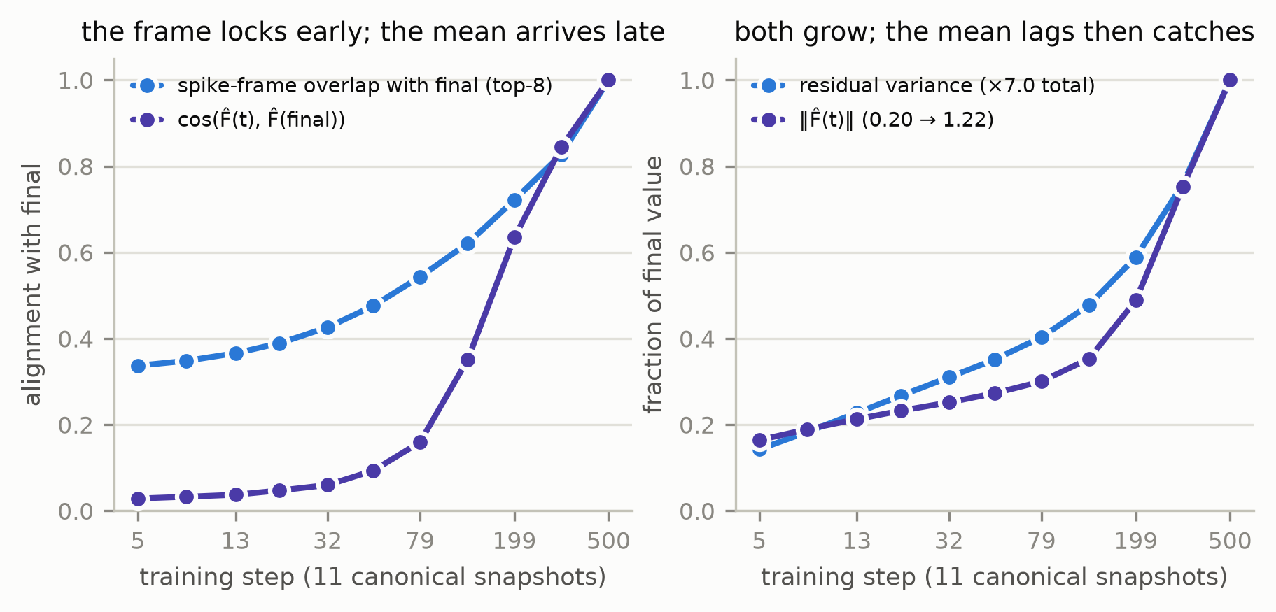
Along the 11-snapshot trajectories (Figure 12), the law and the mean move on different clocks. The spike frame is fixed early and rotates smoothly into its final configuration — mean top-8 subspace overlap with the final frame climbs 0.34 → 1.00 monotonically — and the spike count is nearly constant (306 → 348) while residual variance grows ×7.0 (37.3 → 261.4). The mean is the late arrival: cos(F̂(t), F̂(final)) sits at 0.03 at the earliest snapshot, is still at 0.35 by step 126, and crosses 0.5 only around step ~160 of the 500-step run (between the eighth and ninth of the eleven log-spaced snapshots), while ‖F̂(t)‖ grows 0.20 → 1.22. Training, in this chart, first fixes where the population’s variance will live, then grows the shared signal inside it.

5.2 The atoms are the chart’s coin flips: a measured gauge artifact, repaired on the record

The registered atomicity test asked whether a continuous density is even the right object for the seed-ensemble law. The verdict rule — maximum k-means silhouette above the q95 of 32 matched-Gaussian nulls — fired: silhouette .0223 > .0178, k = 2, a 655/369 split. The population is ATOMIC in the standard chart.

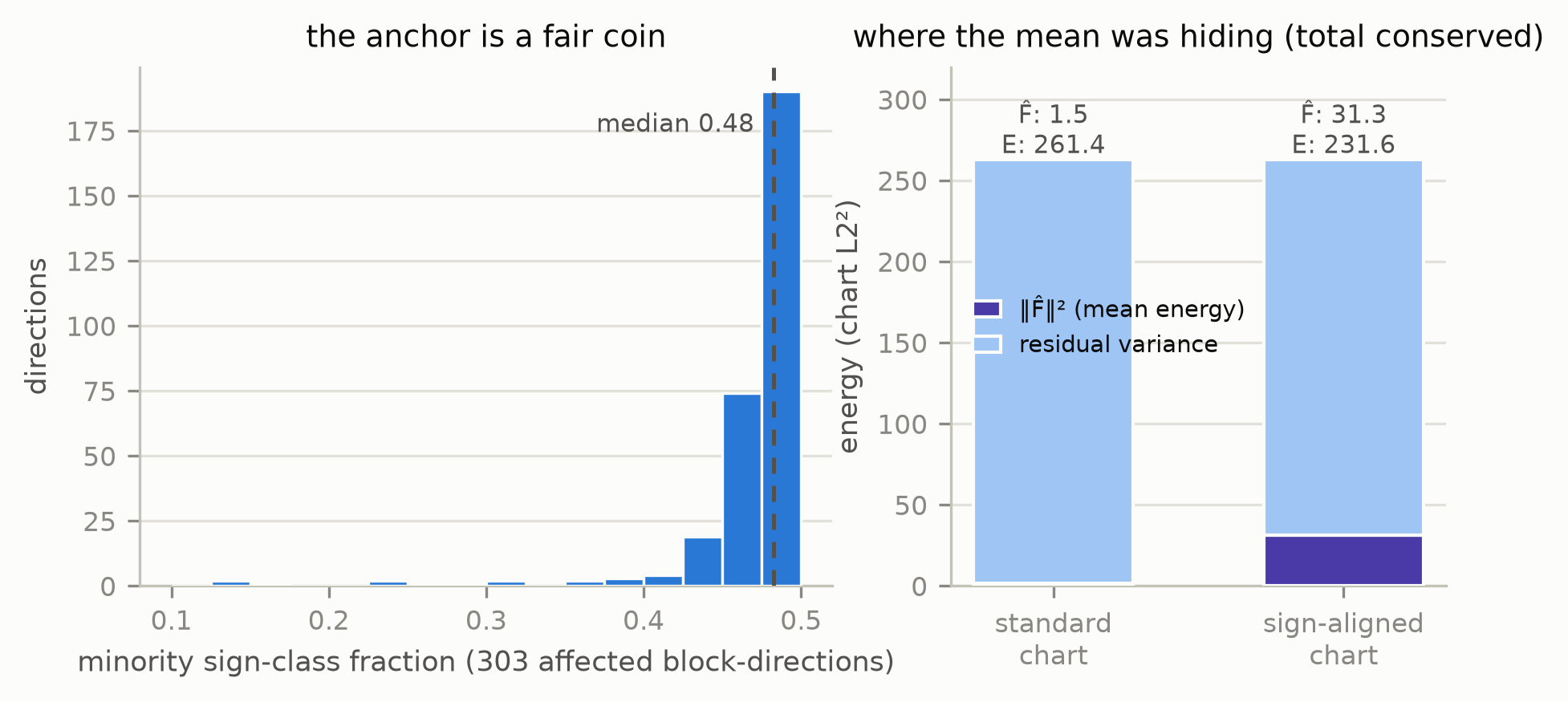
Then the mechanism turned the finding inside out (Figure 13). The split lives on the global first principal component, 54% of whose energy sits in a single block; the two mode means are antipodal (cosine −0.9969 and −0.9930 on the top factor directions) — exactly the (u, v) → (−u, −v) two-element residual gauge of an SVD factorization; and every gauge-invariant statistic of the two modes is identical (singular values within .07 sd, accuracy .8389 vs .8384, era-uniform membership). The cause is the canonical chart’s sign anchor (argmax |v|): on directions whose anchor coordinate is not dominant — the anchored entry holds a median 11% of the direction’s norm — the convention assigns the ± class effectively by coin flip. The measured prevalence: 303 (block, direction) pairs among the top factor directions, with a minority class holding a median 48% of the population — a fair coin, flipped per-model.

The indeterminacy itself is classical: factor analysis has long known that SVD signs are arbitrary and must be fixed by a data-driven convention before factors can be compared or aggregated (Bro et al., 2008), and the LoRA weight-space literature has noted the residual sign flip of SVD canonicalization as a uniqueness caveat (Putterman et al., 2025). What appears to be new is the population-level phenomenon: the convention’s classes measured as coin flips across independently trained models, the mean’s energy cancelled by them, and a registered mixture verdict traced to the chart. The repair is also not TIES-Merging’s sign election (Yadav et al., 2023): their sign conflicts are genuine cross-task disagreement in raw coordinates, resolved by discarding minority contributions; ours are same-task chart artifacts, and every flip is an exact function-preserving gauge move that discards nothing.

The consequences for the mean field are large. Majority-anchored re-alignment (the flip map is banked and deterministic; every flip is an exact ΔW-preserving gauge move, so nothing about any model’s function changes) raises ‖F̂‖ from 1.224 to 5.597: sign mixing had cancelled ~95% of the mean’s energy along the shared directions. The bookkeeping is exact — total residual variance drops 261.44 → 231.62, and the difference (29.83) equals ‖F̂_al‖² − ‖F̂‖² to numerical precision — and the law is untouched: spike counts are unchanged under alignment (347.9 vs 347.6), and the population is exchangeable in the aligned chart (registered split tests p = .33, .13). Functionally, the standard-chart F̂ evaluates at .653 — the zero-adapter task floor: the naive population mean of this corpus does nothing, not because the population lacks a mean but because the chart was averaging sign classes against each other.

This forced the campaign’s one amendment. The ratified design pinned the standard chart; Stage 1 measured that convention to be leaving a two-element gauge unquotiented on 303 shared directions. Both coherent branches were put on the record — render in the sign-aligned chart, or implement the registered mixture re-scope literally in the standard chart (which would model a measured gauge artifact as structure and center every render on a functionally-collapsed mean) — and the operator ratified Branch ALIGNED before any render was materialized. Rungs 1–4 and the comparator fit and render in the aligned chart; F̂ for renders is the same coordinate-wise-mean estimator computed after quotienting the measured discrete gauge; the raw-chart controls, the corpus, the τ ladder, and every incumbent are untouched. The registered reserve clause (mixture families on an ATOMIC verdict) is thereby discharged by mechanism: the atoms are gauge, not structure.

The instrument note, published in the house tradition: the literal registered atomicity statistic — an energy-distance permutation test between random halves — is null-by-construction (random halves are themselves null draws; a smoke test with a planted blatant mixture read p = .83, recorded as a construction pin in the gate-3 addendum), and its observed p = .66 is reported as registered but carries no verdict. The verdict is carried by the silhouette-against-matched-nulls rule, which the smoke test validated, and the energy-distance machinery is applied where it is informative: the structured exchangeability splits above. An audit whose instruments go unaudited is theater; this one caught both a defective statistic and a defective chart before either could touch a render.

5.3 The realization is the init: Rainbow dynamics hold in adapter space, in a stronger form (P-A5-4)

The Rainbow dynamics claim — training learns the law while the noise realization is preserved from initialization — is directly falsifiable on this zoo: we hold every init seed. The registered test regenerates each lineage’s init from its seeded build path (regeneration gate: cosine .9995 against real stored near-init rows), fits the per-block law on raw-chart A-factor residuals (the init exists only in the raw gauge: B = 0 at init makes the canonical quotient degenerate there), whitens each trained adapter, and compares against its own init under a paired-cosine statistic with a shuffled-pair null.

P-A5-4 confirmed, decisively: whitened paired cosine median 0.957 against a shuffled null of −0.001 (registered rule: > 0.3 / < 0.05); the near-init positive control reads 0.999. The sharpening is that whitening is barely needed: the unwhitened paired cosine is 0.956. In adapter space the claim holds in a stronger form than its CNN original — the A-side residual realization simply is the init realization to ~90% of its energy, with training parking learned content in B and a ~9% A-drift. Fine-tuning, on this corpus, is not re-drawing the noise; it is coloring the draw it was given.

Note what the render ladder then showed: this init-anchoring of the population’s realizations places no constraint on renders — free draws from the described law pass everywhere (§5.5). The realization is the init; the law neither knows nor cares.

5.4 Tolerance is anisotropic, and the population mean is variance-collapsed (the registered panel)

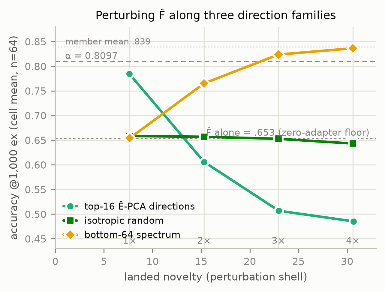
The Feng–Tu tension — SGD fluctuation variance concentrates in sharp directions, so shouldn’t residual-directed noise kill accuracy? — was adjudicated with a registered twelve-cell panel before any rung fired: perturb F̂ along three direction families (top-16 Ê-PCA, isotropic random, bottom-64 spectrum) at matched novelty shells, with an F̂-alone control point (Figure 14).

The control point anchors everything: acc(F̂) = .653, the zero-adapter floor (§5.2’s functional collapse, measured directly). From there:

• Top-PCA directions kill monotonically: .784 / .606 / .507 / .485 at 1–4×. Population variance does concentrate in low-tolerance directions — the Feng–Tu sign, read in our chart at the across-seed level.
• Isotropic noise is amplitude-invariant at the floor: .658 / .657 / .653 / .643 from 1× to 4×. Random directions neither restore nor destroy; the collapsed center stays collapsed.
• Bottom-spectrum directions RESTORE function with amplitude: .654 → .765 → .824 → .836, reaching 63/64 and 64/64 α-passers at 3× and 4× with φ-pass 1.000 — N&P&F 1.000 at the 3× view. Perturbation is not a tax the render pays; along the right directions it is the repair that gives the collapsed mean back its variance.

The panel reshaped expectations on the record (the gate-3 addendum notes “P-A5-3’s premise is already under strain”): a fully described construction — the mean plus scaled bottom-spectrum content — was already reaching the σ-push class before the ladder fired. It also disposes of the naive Feng–Tu reading for renders: what matters is not that variance lives in sharp directions, but that the complement of the population’s variance directions is where amplitude is free.

5.5 The render verdict: the quotient is load-bearing, and describability saturates the audit (P-A5-1, P-A5-2)

The registered grid: 24 cells — rungs 0a/0b at their reachable shells, rungs 1–4b and the comparator at 2×/3×/4× (1× is unreachable for centered cells; the F̂_al floor, §4) — 64 seeded draws each, evaluated at 1,000 examples, with two full-test flagships selected by a rule registered before any evaluation (the rule is fixed pre-eval; which cells it picks is, by construction, a result). The N&P&F verdict surface is Figure 15; the spine, at each cell’s targeted shell:

family	2×	3×	4×	acc mean at 4× (max)
0a raw-chart Gaussian (Zeng control)	—†	0.000	0.000	.653 (.664)
0b ball around one adapter	0.000	0.000	0.000	.813 (.838)
1 white, per-block variance	0.516	0.656	0.672	.817 (.829)
2 sampled colored covariance	0.203	0.594	0.688	.837 (.852)
3 elliptical + empirical radius	0.672	0.688	0.562	.841 (.856)
4a spectral-split	0.484	0.594	0.688	.816 (.828)
4b + frozen small-SV tail	0.500	0.812	0.781	.815 (.828)
empirical-Ê comparator	0.016	0.000	0.000	.689 (.766)

† Raw-chart 1×/2× cells are unreachable-as-targeted (the raw-chart construction’s own novelty floor sits at ≈ 22.9 — the raw chart is that far from its own corpus); recorded, and the reachable cells land on-shell.

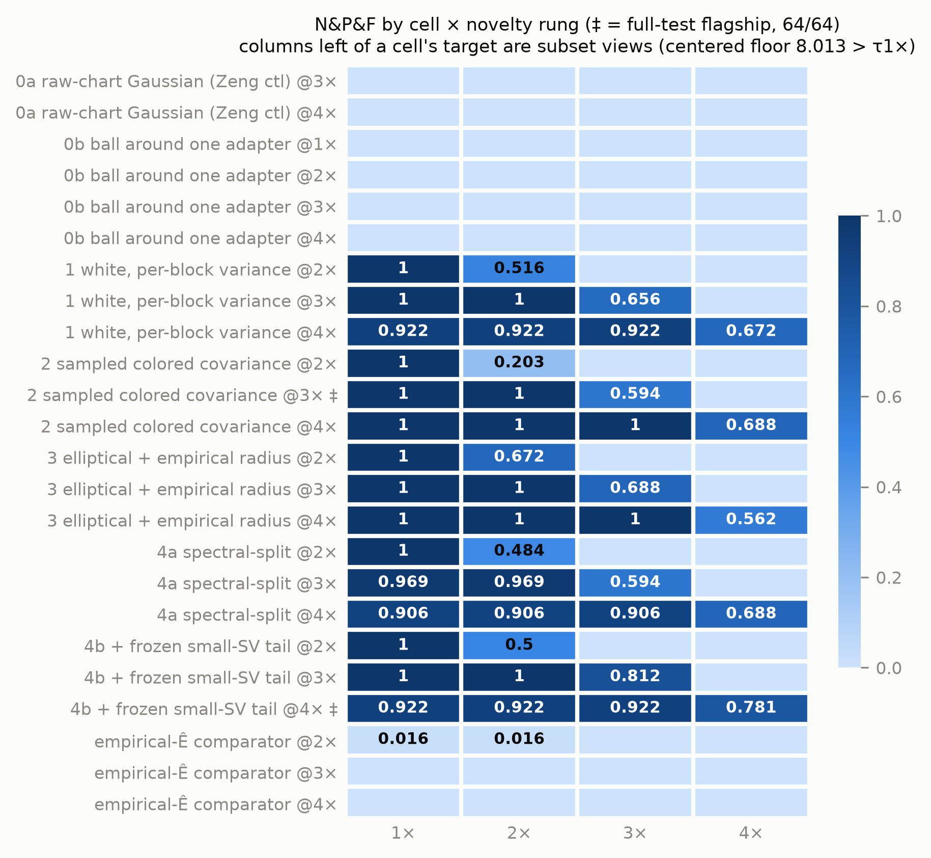
Reading the controls first:

• P-A5-1 (the quotient is load-bearing): CONFIRMED. The rung-0a control — Zeng’s own statistics-only baseline, reconstructed as registered — produces zero passers of any kind at every landed shell, with accuracy pinned at .653: the raw-chart mean is as functionally collapsed as the standard-chart canonical mean, and per-dimension raw statistics render nothing but the floor. Rung 2 exceeds it on every metric component (at the 1× subset view: N&P&F 1.000 vs 0.000, accuracy .841 vs .653). The entire distance between “statistics fail” (the published prior) and “statistics saturate” (this paper) is the quotient plus the population plus the audit.
• The trivial law is hollow, exactly as the filter predicts. Rung 0b — the isotropic ball around one adapter — keeps accuracy at every shell (.813–.818 mean, up to 64/64 α-passers) and scores φ = 0.000 everywhere: noise inherits the function of what it perturbs, so a ball around one member is a factory of functional clones of that member at arbitrary geometric distance. Every one of its 212 α-passers across the four shells is caught by the functional filter. Without φ, rung 0b would read as a saturating “generator” — the audit’s sharpest illustration yet of why geometric novelty alone is gameable.

Then the described families:

• P-A5-2 (describability): CONFIRMED beyond its bar. The registered bar was N&P&F ≥ 0.9 at 1× for at least one of rungs 2–4. Multiple rungs hold 1.000 at the 1× and 2× subset views (with the subset-view caveat of §4 attached to both), every rung 1–4b passes φ at rate 1.00 in every cell — fresh draws from the described laws are functionally distinct from every corpus member, not just geometrically far — and the deep cells (§5.6) render the bar moot.
• The flagships confirm at full test. By the registered rule (best described rung at 1×; deepest cell with any described passer): rung 2 at the 3× shell — 64/64 above α on the full 3,270-example set, mean .8427, max .8511; rung 4b at the 4× shell — 64/64, mean .8207, max .8309. (Several rungs tie at 1.000 on the 1× view; the banked selection of record is rung 2, a5-verdict.json — the tie itself is §5.7’s finding.) For calibration: the corpus members’ own mean is .839 (the Stage-1 addendum’s member baseline). Described renders at three times the population’s spread are, at full test, member-indistinguishable; at four times, within two points of it — and the best rendered adapter at 1,000 examples (.856, a rung-3 row at the 4× shell) and the best at full test (.851, in the rung-2 flagship) both exceed the member mean.

5.6 The inversion: described laws beat the population’s own realizations (P-A5-3)

P-A5-3 predicted the deep frontier is realization-bound: no described rung produces any N&P&F passer at ≥ 3×, while the empirical-Ê comparator — the population’s own residuals, freshly paired and rescaled, the factor-chart image of the previous paper’s σ-push recipe — passes there. Any described 3× passer would falsify it.

P-A5-3 is FALSIFIED — INVERTED. The described rungs pass at depth in abundance (best N&P&F 1.000 at 3×, 0.781 at 4×), while the comparator produces zero α-passers at 3× and 4× (accuracy means .760 and .689, maxima .809 and .766 — both under the bar) and only a single φ-passing row at 2× (pass fraction 0.016; of its 26 α-passers there, 25 fail the functional filter). The registered centerpiece statistic, the described-minus-empirical delta in N&P&F pass fraction at matched shells:

shell	best described (source cell)	empirical-Ê comparator	delta
1× (view of the 3×-target cell)	1.000 (rung 4b @3×)	0.016	+0.984
2× (view of the 3×-target cell)	1.000 (rung 4b @3×)	0.016	+0.984
3× (view of the 4×-target cell)	1.000 (rung 3 @4×)	0.000	+1.000
4× (at target)	0.781 (rung 4b @4×)	0.000	+0.781

The campaign was designed to price the cost of describing the residual rather than carrying its realizations; the price came back negative at every shell. Two mechanisms, both already measured, compose to explain it:

1. Scaling a realization is radial extrapolation along one draw. The comparator at shell c is F̂_al + c·Ê_i — one member’s residual, amplified. The previous campaign measured extrapolation along member-defined directions to cliff after 3× while orthogonal pushes ride free; the comparator’s accuracy profile (.806 → .760 → .689 as c grows) is that cliff, reproduced in the factor chart. A fresh draw from the described law at the same shell spreads its mass across the law’s whole support — mostly the high-tolerance complement (§5.4) — and never concentrates its distance along any single low-tolerance realization.
2. A scaled member-residual stays functionally its member. The comparator’s φ collapse at 2× (0.04 φ-pass among α-passers) is rung 0b’s lesson in population clothing: c·Ê_i points back toward member i, and the render computes nearly member i’s function — geometrically far, functionally home. Described draws pass φ at 1.00 in every cell.

The nearest comparison on record points the opposite way and does not conflict: around single deep-ensemble members at native scale, sampling fitted local Gaussians does not beat the members themselves (Jordahn et al., 2025). That is a 1× comparison with no amplitude push — the regime where our comparator is also healthy. The inversion is a deep-shell phenomenon: it appears where rescaling forces a single realization to extrapolate, a regime the ensemble literature never enters.

The previous paper’s deep-frontier result carried the population’s own noise and survived because its base was a functionally-novel soup and its push was orthogonal. This campaign’s finding is stronger and simpler: at matched construction — same center, same shells, same chart — the described law is not a cheap approximation of the empirical residuals; it is the better noise. The deep frontier is not realization-bound. It is realization-hostile.

5.7 The hierarchy is flat: variance is the description (and two published disputes, adjudicated at the bar)

Reading Figure 15 across rungs rather than down shells: at the deep readings — the 3× and 4× targets, and every deeper cell’s shallower views — rung 1 (white Gaussian at matched per-block variance) sits within noise of rungs 2, 3, 4a, and 4b (at the 4× target: 0.672 / 0.688 / 0.562 / 0.688 / 0.781 across the five; n = 64 per cell; at the 3×-cells’ 2× views: 0.97–1.00 across all five). The at-target 2× column is the one place the rungs visibly spread (.203–.672) — and it is landing jitter, not law difference: an at-target cell’s rows sit on their own rung boundary, so sub-percent landing error flips rows across the threshold (rung 2’s 2× cell landed at median 15.272 against a boundary of 15.297 — §5.8); the same rungs read 1.000 together one row deeper. The added structure each deeper rung encodes — the sampled colored covariance (hundreds of above-edge eigenpairs per block), the empirical radial law, the deterministic spike head, the frozen small-SV tail — buys nothing the audit can measure. The render-relevant description of this population is (aligned mean, per-block variance): the mean field, one residual variance per matrix block — 196 scalars of law, all the law there is — and the flip map that makes the mean well-defined.

This lands on two published disputes at once:

• Rainbow vs. Martin–Mahoney (covariance-correlations vs. power-law readings of non-MP spectra) was a registered adjudication at rungs 2 vs 3. The measurement (§5.1) comes back mixed — a spike continuum and mildly heavy tails, neither picture clean — and the render bar declares the question moot at this regime: rung 2 ties rung 3 ties rung 1. Both literatures are describing structure that is really present in Ê and really unnecessary for rendering function. The dispute, at least here, is about the residual’s portrait, not its use.
• The Zeng verdict inverts under the quotient. The field’s referee showed learned generators failing to beat raw per-dimension Gaussians — and concluded the generators memorize. Our rung 0a shows those same raw Gaussians render nothing; our rung 1 shows the identical parametric family, fitted in the quotiented aligned chart, saturates the deep audit. The statistics were never the problem, and the generators were never the point: the chart was both.

What, then, did learning buy? On this scoreboard (incumbents by reference): the weight-space flow reached 0.004 at 1× and nothing deeper; the learned recombiner tied the soup on N&P at 1×/2× (1.000/1.000; under N&P&F it scored .953, three φ-marginal rows short of the soup — the previous paper’s two-level verdict, kept uncollapsed here as there) and sampled three deep objects by conditioning leakage; the σ-pushed soups — a fixed operator with a described scale — saturated 3×/4× (N&P&F 1.000 at both) carrying empirical residuals in the ΔW chart. The described families reach every shell those operators reach, with no training, no GPU in the fit, and a residual law that fits on an index card — matching the incumbents’ saturation through 3× and trailing only the σ-push’s 1.000 at 4×, where the best described cell holds 0.781. What none of the described families has is the recombiner’s dial: accuracy-conditioned steering (ρ = .781) remains the one measured capability unique to a learned generator in this series. Learning bought steering. Reach belongs to statistics.

5.8 Instrument notes

In the series tradition, the campaign’s instrument record, in the open: the atomicity statistic that was null-by-construction (caught by smoke test, verdict re-carried by the calibrated silhouette rule, §5.2); the threshold sensitivity of at-target pass fractions (an at-target cell’s rows land on their own rung boundary, so the at-target 2× column of Figure 15 is dominated by sub-percent landing jitter — §5.7 — while deeper cells’ views are jitter-free); the comparator’s landed shells bending across target (medians 18.30 / 23.65 / 28.96 against 15.30 / 22.95 / 30.59 — over at 2×/3×, under at 4× — its calibration was fitted in the natural (c−1)² variable, but amplification switches some rows’ nearest corpus neighbors; per-row landed novelty carries the adjudication, so the bend costs headroom rather than validity: it helps the comparator at 2×, where its landed median overshoots the target, and shaves the 4× rung, where it under-lands); and the raw-chart control’s nearest neighbors, which required an explicit raw→canonical row mapping so that φ could be scored against the correct corpus predictions. Every cell’s draws regenerate from banked manifests; the spectral frames are environment-pinned (eigendecompositions re-certified after any BLAS change before regeneration is trusted).

6. Limitations

Regime-boundedness, first and always. One base model (Qwen3-0.6B, revision-pinned), one task (BoolQ), one rank (r=8), seed-only variation. The previous campaign’s extinction-law lesson — a clean law that declined to generalize one regime over — is the standing prior for every strong claim here. “The render-relevant description is mean plus variance” is a measured fact about this population; whether describability survives mixed provenance, task variation, rank variation, or base-model scale is exactly the firewalled Stage-4 question, untested by design. The 6× novelty rung was never targeted. The comparator is one construction (scaled single-member residuals with fresh pairings); richer empirical-residual recipes (mixtures of members’ residuals, init-anchored draws per §5.3) were not registered and were not run.

The chart caveat, in full (the §A.4 obligation, restated from §4): A5’s novelty numbers are chart L2 distances to the stored unaligned corpus. Sign alignment displaces aligned-chart objects by ~14 (median member displacement 14.05) relative to that stored corpus, so: 1× is a subset view by construction (the centered floor is 8.013 > τ1×); 2× novelty (15.30) is only modestly beyond the displacement scale; and A5 novelty values must not be compared against aligned-chart distances without saying so. The claims that carry the campaign — accuracy, φ, the 3×/4× shells at 1.6–2.2× the displacement, and the described-vs-empirical delta (same chart both sides) — are either chart-free or displacement-matched. We publish the displacement number rather than an aligned-corpus re-index because the stored corpus is the registered referee every incumbent was scored against; re-indexing mid-campaign would have broken the one-scoreboard property that makes the delta meaningful.

What the flat hierarchy does not say. Rungs 2–4b tie rung 1 at n = 64 per cell; a single 64-draw cell carries a ±0.12 (2σ) uncertainty on its own pass fraction, and a difference between two such cells resolves only at roughly ±0.17 — and the flatness claim is scoped to the deep readings, where at-target threshold jitter is absent (§5.7). Structure that matters at finer resolution — or at shells, tasks, or bases we did not probe — would need bigger cells to surface. The claim is “nothing measurable at this audit’s resolution,” not “nothing.”

On generalization. As throughout the series: no claim here concerns generalization of rendered adapters beyond the audited task, and novelty is scored in function space precisely because geometric novelty alone is gameable (§5.5). Rendered adapters are new functions that pass the task’s bar; they are not certified to be good at anything else.

7. Discussion

The series’ through-line sharpens by one more step. Paper 1: fixing the coordinates makes honest generation possible. Paper 2: the frontier belongs to operators that respect the population’s geometry, and a learned generator can own the operator. This paper: once the coordinates are fully fixed — including the discrete convention this campaign caught mid-flight — the density that remains is so simple that a mean and a variance table render member-grade, functionally-novel weights at four times the population’s spread. In this regime, the entire difficulty of “generative models of weights” was coordinates. There was almost no density left to learn.

The inversion is the finding we least expected and the one we now find most natural. The intuition “the population’s own residuals are the gold-standard noise; a fitted law is a lossy stand-in” has it exactly backwards at depth, for a reason the previous campaign already measured without naming: a realization is a direction, and amplified directions exit the basin; a law is a distribution, and its fresh draws put their mass where the tolerance is. Description is not the cheap approximation to resampling — at depth, it is the only one of the two that works.

The sign-class episode deserves its own moral. The atomicity instrument was registered to test whether a continuous density was the right object, with a mixture-family re-scope armed if not. It fired — and the mechanism showed the atoms were the chart’s own coin flips, hiding 95% of the mean’s energy, with the “population mean” every naive analysis would compute sitting at the task floor. Canonicalization is not a checkbox: a convention (which sign survives an SVD) is as much gauge as a rotation is, and it becomes load-bearing exactly when a population is averaged across it. We suspect this failure mode is quietly present in other weight-population statistics; any pipeline that averages SVD factors across independently-trained models should check its anchors’ stability before trusting its means. (The hazard is live: of the SVD-based weight-space pipelines our citation walk examined, those not structurally immune by joint factorization carry no sign treatment at all.)

The rainbow-dynamics confirmation places adapter fine-tuning in an unexpectedly clean corner of the Guth et al. picture: the realization is the init to ~90% energy — stronger than the CNN original — while the law’s frame locks in early and the mean arrives late. Training, seen from weight space, is here almost entirely a coloring process. And yet the renders show the init-anchoring binds only the population, not the family: free draws function. The law is the object; the realizations, including the inits, are merely where this particular population happens to have sampled it.

What should a practitioner take? For this task, rendering a functionally novel, member-grade adapter costs: one aligned mean, 196 variances, a seed, and a scale — no training, no GPU. What should the field take? The referee literature’s “generators fail to beat cheap statistics” and this paper’s “cheap statistics saturate the audit” are the same fact seen from two charts: the baseline was never weak, it was mis-coordinatized — and the learned-generator question should be re-asked after the quotient, where the honest answer, at least here, is that learning contributes steering, not reach. The open question the series now walks toward is the one the flat hierarchy poses: if a mean and a variance table suffice at one (base, task, rank), what is the smallest description that survives varying them — and does the gap between described and learned stay closed when the population stops being seed-pure? That is Design-B territory, firewalled out of this campaign, and the natural fourth question.

8. Reproducibility statement

The campaign ran from a pre-registered design ratified before firing (journal entry 085), with Stage-1 verdicts and construction pins recorded as a dated addendum before any render materialized (gate 3), one operator-ratified chart amendment on the record before the grid fired (§A.4), a registered 24-cell grid with no post-hoc cells (gate 4), and adjudication of all four predictions plus the centerpiece delta on the record (gate 5; journal entries 086–090). Every fit, render, calibration, and scoring tool is in the repo (.research/a2-ops/a5_battery.py, a5_panel.py, a5_render.py); canonical numbers ship as the JSON artifacts named throughout; every render cell carries a seeded draw manifest; evaluation labels are alignment-asserted per job; novelty preseeds are CPU-computed and verified against banked values; the sign-alignment flip map is banked and deterministic; spectral frames are environment-pinned with re-certification required after numerical-stack changes. The zoo build, sidecar evaluation machinery, corpus, bars, and incumbent artifacts are those of the previous papers, unchanged.

References

(Assembled from the verified bibliographies of papers 1–2 — items marked ◆ carry over — plus the 2026-08-23 five-lens EFG literature wave. Re-walked pre-publication, 2026-08-27, by three parallel sweeps: every entry verified against its arXiv/proceedings/publisher record; a scoop sweep on the headline claim (none found — the statistics-only branch remains unoccupied, including in the field’s own 2026 position-paper taxonomy); and a prior-art sweep on the §5.2/§5.6 discoveries (not scooped; the classical sign-ambiguity line and the nearest ensemble comparison added and distinguished inline).)

The series

1. Canonicalize, Then Generate: Quotienting Weight-Space Symmetries Unlocks Honest Generative Models of Neural Network Weights. Haphazard Solutions lab publication, 2026. haphazardsolutions.com/knowledge/canonicalize-then-generate/.
2. Recombine, Then Generate: A Pre-Registered Audit of Weight-Space Merging and the Deep Novelty Frontier in LoRA Adapter Populations. Haphazard Solutions lab publication, 2026. haphazardsolutions.com/knowledge/recombine-then-generate/.

The premise’s nearest neighbors

1. Guth, Ménard, Rochette, Mallat. A Rainbow in Deep Network Black Boxes. JMLR 25 (2024). arXiv:2305.18512. — the premise executed on CNNs: colored Gaussian layers, activation-Procrustes alignment, rendered networks, the law-vs-realization dynamics finding; distinguished in §2.
2. Xiao, Liu, Bamler. A Compact Representation for Bayesian Neural Networks by Removing Permutation Symmetry. UniReps Workshop @ NeurIPS 2023. arXiv:2401.00611. — the rebasin-then-moments move at workshop scale.
3. Maddox, Izmailov, Garipov, Vetrov, Wilson. ◆ A Simple Baseline for Bayesian Uncertainty in Deep Learning (SWAG). NeurIPS 2019. arXiv:1902.02476.
4. Immer, Korzepa, Bauer. Improving Predictions of Bayesian Neural Nets via Local Linearization. AISTATS 2021. arXiv:2008.08400. — the standing negative on sampling fitted weight posteriors.
5. Bolager, Burak, Datar, Sun, Dietrich. Sampling Weights of Deep Neural Networks (SWIM). NeurIPS 2023. arXiv:2306.16830. — render-without- training from a data-derived law.
6. Fortuin, Garriga-Alonso, Ober, Wenzel, Rätsch, Turner, van der Wilk, Aitchison. Bayesian Neural Network Priors Revisited. ICLR 2022. arXiv:2102.06571.

Referees and controls

1. Zeng, Yin, Xu, Liu. ◆ Generative Modeling of Weights: Generalization or Memorization? CVPR 2026 (Highlight). arXiv:2506.07998. — the memorization referee whose statistics-only control is our rung 0a.
2. Gupta, Biggs, Laber, Shafi, Walters, Paul. ◆ DeepWeightFlow: Re-Basined Flow Matching for Generating Neural Network Weights. ICLR 2026. arXiv:2601.05052.
3. Shi, Wang, Han, Zhang, Wang. Training-Free Bayesianization for Low-Rank Adapters of Large Language Models (TFB). NeurIPS 2025. arXiv:2412.05723. — the isotropic ball-around-one-adapter construction behind rung 0b.
4. Gan, Isola. Neural Thickets: Diverse Task Experts Are Dense Around Pretrained Weights (RandOpt). ICML 2026 (Spotlight). arXiv:2603.12228. — training-free but selection-powered; distinguished in §2.
5. Z. Wang, P. Wang, K. Wang. ◆ Position: Weight Space Should Be a First-Class Generative AI Modality. ICML 2026 (Position Paper track), PMLR 306. arXiv:2605.18632.

Weight statistics, spectra, and geometry

1. Martin, Mahoney. Implicit Self-Regularization in Deep Neural Networks: Evidence from Random Matrix Theory and Implications for Learning. JMLR
   1. arXiv:1810.01075. — the heavy-tailed reading adjudicated at rungs 2 vs 3.
2. Jang, Yun, Han. ◆ Model Stock: All We Need Is Just a Few Fine-Tuned Models. ECCV 2024. arXiv:2403.19522. — the thin-shell/center geometry, measured in our chart in §5.1.
3. Rame et al. ◆ Diverse Weight Averaging for Out-of-Distribution Generalization (DiWA). NeurIPS 2022. arXiv:2205.09739.
4. Jordan, Sedghi, Saukh, Entezari, Neyshabur. REPAIR: REnormalizing Permuted Activations for Interpolation Repair. ICLR 2023. arXiv:2211.08403. — the variance-collapse lesson; §5.2, §5.4.
5. Feng, Tu. The Inverse Variance–Flatness Relation in Stochastic Gradient Descent Is Critical for Finding Flat Minima. PNAS 118(9):e2015617118,
   1. — adjudicated by the §5.4 panel.
6. Dinh, Pascanu, Bengio, Bengio. Sharp Minima Can Generalize for Deep Nets. ICML 2017. arXiv:1703.04933. — sharpness is chart-dependent.
7. Staats, Thamm, Rosenow. Small Singular Values Matter: A Random Matrix Analysis of Transformer Models. arXiv:2410.17770. — the low-σ tail trap behind rung 4b.
8. Pittorino, Ferraro, Perugini, Feinauer, Baldassi, Zecchina. Deep Networks on Toroids: Removing Symmetries Reveals the Structure of Flat Regions in the Landscape Geometry. ICML 2022, PMLR 162:17759–17781; also J. Stat. Mech. 114007 (2022), doi:10.1088/1742-5468/ac9832. arXiv:2202.03038. — the quotient is not a vector space.
9. Hu, Goel, Killiakov, Yang. Eigenspectrum Analysis of Neural Networks without Aspect Ratio Bias (FARMS). ICML 2025. arXiv:2506.06280.
10. Loaiza-Ganem et al. Deep Ensembles Secretly Perform Empirical Bayes. arXiv:2501.17917. — the atomic-law falsifier engaged in §5.2.
11. Jordahn, Jensen, Schmidt, Andersen. On Local Posterior Structure in Deep Ensembles. AISTATS 2025, PMLR 258:5032–5040. arXiv:2503.13296. — fitted local Gaussians do not beat the members at native scale; distinguished at §5.6.
12. Kaushik, Chaudhari, Vaidya, Chellappa, Yuille. The Universal Weight Subspace Hypothesis. arXiv:2512.05117. — shared spectral subspaces across model and adapter populations; description without rendering.

Gauge, alignment, and mode connectivity

1. Bro, Acar, Kolda. Resolving the Sign Ambiguity in the Singular Value Decomposition. Journal of Chemometrics 22(2):135–140, 2008. doi:10.1002/cem.1122. — the classical statement and data-driven repair of SVD sign indeterminacy; engaged at §5.2.
2. Entezari, Sedghi, Saukh, Neyshabur. ◆ The Role of Permutation Invariance in Linear Mode Connectivity of Neural Networks. ICLR 2022. arXiv:2110.06296.
3. Ainsworth, Hayase, Srinivasa. ◆ Git Re-Basin: Merging Models modulo Permutation Symmetries. ICLR 2023. arXiv:2209.04836.
4. Crisostomi et al. C²M³: Cycle-Consistent Multi-Model Merging. NeurIPS 2024. arXiv:2405.17897. — the universe-frame instinct for putting a whole zoo in one gauge.
5. Putterman, Lim, et al. Learning on LoRAs: GL-Equivariant Processing of Low-Rank Weight Spaces for Large Finetuned Models. ICLR 2025. arXiv:2410.04207. — notes the residual sign flip of LoRA SVD canonicalization as a uniqueness caveat; §5.2 measures its population-level consequence.
6. Yadav, Tam, Choshen, Raffel, Bansal. ◆ TIES-Merging: Resolving Interference When Merging Models. NeurIPS 2023. arXiv:2306.01708. — sign election over genuine cross-task disagreement; distinguished from our gauge flips at §5.2.
7. Zhou, Chen, et al. ◆ Rethinking Diffusion Models with Symmetries through Canonicalization with Applications to Molecular Graph Generation. arXiv:2602.15022.

Generators over this corpus’s lineage

1. Hu, Shen, Wallis, Allen-Zhu, Li, Wang, Wang, Chen. ◆ LoRA: Low-Rank Adaptation of Large Language Models. ICLR 2022. arXiv:2106.09685.
2. Wortsman et al. ◆ Model Soups. ICML 2022. arXiv:2203.05482.
3. Lipman, Chen, Ben-Hamu, Nickel, Le. ◆ Flow Matching for Generative Modeling. ICLR 2023. arXiv:2210.02747.
4. Peebles, Radosavovic, Brooks, Efros, Malik. ◆ Learning to Learn with Generative Models of Neural Network Checkpoints (G.pt). arXiv:2209.12892.

The information-theoretic frame

1. Havasi, Peharz, Hernández-Lobato. Minimal Random Code Learning: Getting Bits Back from Compressed Model Parameters. ICLR 2019. arXiv:1810.00440.
2. He, Flamich, Hernández-Lobato. Getting Free Bits Back from Rotational Symmetries in LLMs. arXiv:2410.01309.
3. Lamaakal. Motion-Compensated Weight Compression (MCWC). arXiv:2605.24754. — the compression-side twin: aligns the gauge, predicts F, codes E, never samples it.

Field surveys and adjacent lines

1. Han, Wang, Zhao, Zhang, Li, Borth, Yu, Maron, Ye, Yin, Neri. A Survey of Weight Space Learning: Understanding, Representation, and Generation. arXiv:2603.10090. — the field’s own taxonomy, with no statistics-only generation branch.
2. Zhou. Universal Hypernetworks for Arbitrary Models (UHN). arXiv:2604.02215. — weights-as-field with a trained emitter; superficial overlap only.
3. LoRAGen: Structure-Aware Weight Space Learning for LoRA Generation. ◆ ICLR 2026 (OpenReview mrafO7aTYj). — module-indexed spectral statistics observed in the wild, handled with a learned decoder.