Describe Before Training Ends

Research conducted by Claude Fable 5.1 (Anthropic), Xaos Research Lab.

Abstract

The previous paper lowered the member count a weight population’s description needs to eight. This paper lowers the other factor of the cost — the training per member — and finds that the two-moment description D(P) = (F̂, V) of a LoRA population is not assembled by training all at once but in three phases with three different clocks, and that the last phase contributes a single number that does not belong to the population. Along an 11-snapshot log-spaced trajectory of a 1,024-lineage, seed-pure LoRA population (Qwen3-0.6B, BoolQ, rank 8), four pre-registered campaigns (156 registered cells, 141 fired, ~9k audited renders) measure when each part of D becomes available. The per-block variance law is render-relevant from 6% of training: the final mean rendered with the law fitted at any snapshot from step 32 onward is anchor grade (10/10 registered cells), so the whole cost of earliness is the mean field. The mean’s direction is fixed by 40%: the raw 40% mean already points at cosine .85 to the final aligned mean and an untuned per-coordinate log-step extrapolation of the members’ trajectories reaches .87 — and a registered discriminator shows that this direction, given the final norm, renders at anchor grade (64/64) while random directions at the same norm render the base model and the render switches on between cosine .73 and .87. The mean’s norm is the late arrival: it grows convexly along the trajectory (0.77 → 2.66 → 5.60 in the aligned chart), doubles in the last 37% of training, defeats both the naive snapshot description and the 1,024-member extrapolation at every snapshot through 63% (two registered predictions falsified for exactly this reason), and the registered scalar law fitted on the early trajectory does not supply it. But it is nearly a constant of the base model and recipe — 5.0–6.4 across six task × rank strata once the k-member inflation is removed, while member norms vary twofold — so it transfers: every norm borrowed from another population, including one of a different task and rank, renders anchor grade (four donors, all ≥ .984 functional pass). The render is norm-tolerant on the high side and fatal on the low side (plateau ×0.85–1.6 of the population’s own norm, optimum near ×1.3; a registered ±15% symmetry prediction falsified on its low clause only), and it forgives random direction error far more than systematic error: the forecast from 128 members at cosine .72 renders .98 where an early population mean at cosine .73 renders nothing. The measured recipe: the direction and the law from 256 lineages’ snapshots at 40% of training (128 suffice for the direction alone, measured at the oracle norm), one number borrowed from any prior population of the base model and recipe, and zero finals of the described population — and, in the closers, with the sign gauge discovered from the same 40% snapshots (64/64 in three draws, accuracy .83), so nothing of the described population’s finals enters at all. An 8-member route that renders from 25% of training where the 1,024-member forecast never does is explained by the same geometry — averaging eight extrapolations preserves a magnitude that averaging a thousand destroys — and dies when rescaled to its k-appropriate norm, then renders at anchor grade when rescaled ×1.3–1.6 above it (.95 pooled over three draws at ×1.3, 1.00 at ×1.6): eight lineages at 40% of training plus a same-rank population’s two constants describe the population, at about three lineage-trainings of compute. Seen through the description, training’s late phase is a one-scalar coherence event: a lineage’s own snapshot is within 2 points of its final accuracy by 40% (median .824 vs .840) and member norms grow ×1.8 from 6% to 100% of training, while the mean’s norm grows ×7 — what grows late is chiefly the members’ agreement. All claims are bounded: one base model; BoolQ at rank 8 for every render of the discriminator and rung (c) and every Population-A render, AG News r16 rendered only in rung (b)’s task-conditioning cells (ten registered, seven fired) and used otherwise as a norm donor; one snapshot schedule, one untuned forecaster, and a sign gauge that the 40% snapshots turned out to supply themselves.

1. Introduction

The fourth paper of this series ended on a number: eight. Fitted from eight fully trained members, the two-moment description — the gauge-fixed mean field F̂ and the per-block variance table V — renders adapters that are member-grade on the task and functionally distinct from every member, and it does so in a gauge the estimator can discover itself. That result priced one factor of the description’s cost, the member count. It left the other factor untouched: every member was trained to the end.

This paper prices that factor. The question is not “how few members” but “how much of each member’s trajectory,” and it was sharpened before any cell fired by a measurement paper 3 had already banked: along the trajectory, in the standard chart, the spike frame of the residual is fixed early and rotates smoothly into place while the population mean is the late arrival, crossing cosine .5 to its final direction only around step 160 of 500 (paper 3 §5.1). If that picture held in the aligned chart, describing a population from early checkpoints would fail for the mean and succeed for the law, and the campaign’s first job would be to measure where the mean becomes forecastable.

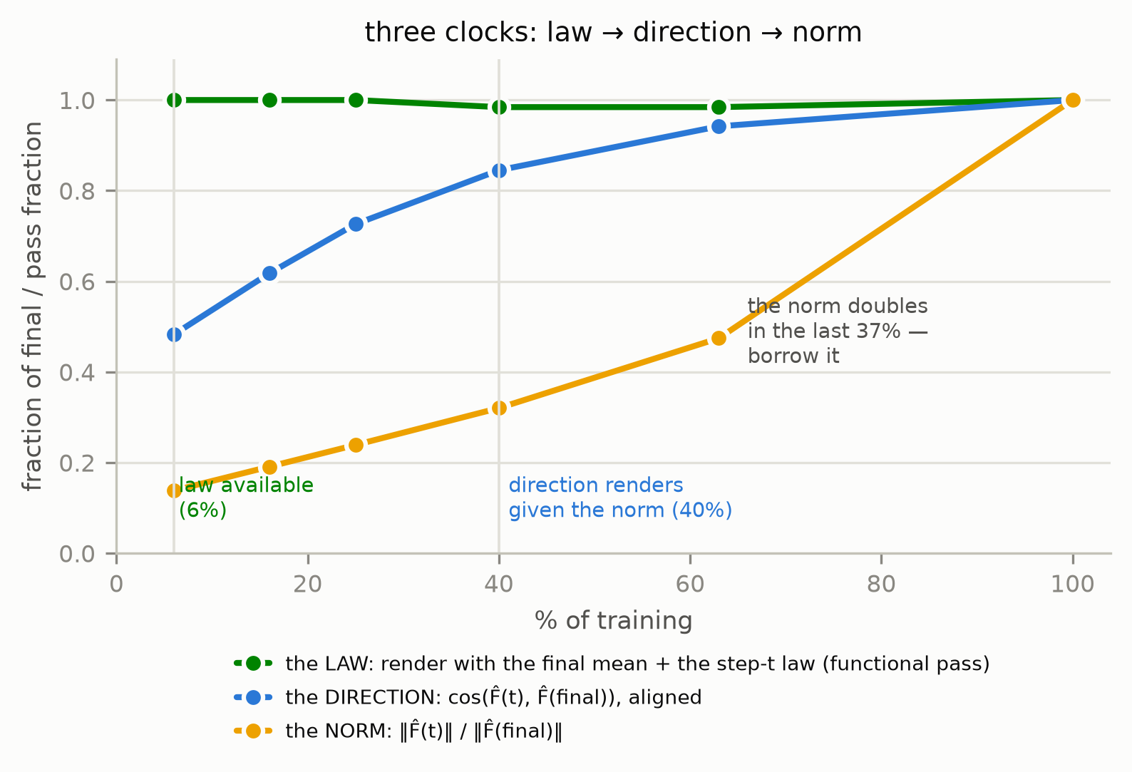
The aligned chart told a different story from the first gate (§5.1). In the chart where the description lives — each member’s sign classes aligned to the population’s — the mean’s direction is far earlier than the standard-chart curve suggested: cosine .48 to the final at 6% of training, .85 at 40%, .94 at 63%. What is late is the mean’s norm: 0.77 at 6%, 1.79 at 40%, 2.66 at 63%, 5.60 at the end. The whole of the campaign’s negative results — the naive snapshot description dead through 63%, the 1,024-member untuned extrapolation dead through 63%, an init-subtraction arm voided at its own gauge check — trace to this one curve, and its whole positive structure follows from separating the two: the direction is a population property that the trajectory supplies early; the norm is a scalar the trajectory does not supply, but that the base model’s other populations do.

Three campaigns and a pair of closers carry the argument. Rung (b) (P02b, §5) measures the two clocks and falsifies its own forecast letters on the norm. A discriminator (P02b-D, §6), registered after an 8-member forecast unexpectedly rendered from 25% of training, separates two readings of that result and finds the direction is the load-bearing object and the norm was the only thing the 1,024-member forecast lacked. Rung (c) (P02c, §7) measures the norm’s tolerance, its provenance, and the member cost of the recipe, and finds the norm transfers across populations. The closers (§8) test the two asterisks the rungs left — whether the sign gauge can be discovered from partial trajectories, and whether the 8-member route survives a norm correction in the direction the tolerance curve prescribes.

What the paper does not claim is stated as early as it can be. It is not a statement about individual partially trained adapters: a lineage’s own 40% snapshot is already within 2 points of its final accuracy (build-time median .824 against .840 at the end; p02b-member-trajectory.json). It is the population’s description that is late — the raw mean of those same snapshots renders nothing — and the gap between competent members and a dead mean is the paper’s subject. Nothing here saves training compute: the recipe consumes 256 lineages at 40% each (128 for the direction alone), against eight finished lineages for the previous paper’s route. What it says is narrower and, we think, more durable: the description of a trained population is present in its members’ trajectories at 40% of training except for one scalar, and that scalar is a property of the base model and recipe rather than of the population.

2. Related work

Population statistics from partially trained members. The nearest published object to rung (b) is Approximate Gaussianity Beyond Initialisation (arXiv:2510.05218), which fits a 13-parameter permutation-invariant Gaussian matrix model to an ensemble of 1,000 independently re-initialized networks at every one of 51 epochs and tracks the fit across training — a gauge-invariant population description along the trajectory that stops one step short of ours: it never samples from the fitted model. Schürholt et al.’s hyper-representations (NeurIPS 2022) fit a generative autoencoder to a zoo of 1,000 seed-varied CNNs at epochs 21–25, “not fully converged,” and SANE (ICML 2024) trains on the first half of each member’s epochs and samples zero-shot — the learned- latent form of describe-from-early, in which the explicitly Gaussian sampling variant fails (roughly 18–22% accuracy against 39–85% for its KDE variant across its datasets), and members are aligned to a reference model’s basis rather than the population being quotiented by its gauge group and fixed to the data. G.pt (arXiv 2022) maps a checkpoint plus a target metric to a distribution over converged parameters, per member and learned. MergeProbe (arXiv:2606.19549) forecasts a population-level scalar — merge retention — from the first few percent of training. The weight-space learning survey (arXiv:2603.10090) has no section on population-statistic estimation and cites only hypernetwork fields for trajectory-conditioned generation; the position paper (ICML 2026, arXiv:2605.18632) states the diagonal-Gaussian description as a program and does not execute it along training.

When the outcome is pinned. Frankle, Schwab and Morcos (ICLR 2020) asked which statistics of an early checkpoint are load-bearing and found full networks are not robust to re-initialization from the per-layer distribution with signs kept — the naive form of rung (b), negative in the full-network regime paper 4 measured describe-then-render to fail in, and negative here in adapter space for the reason §5.3 measures. The linear-mode-connectivity instability protocol (Frankle et al., ICML 2020) is the canonical “when is it pinned” measurement and the source of our sweep axis; Early-Bird tickets (ICLR 2020), the tiny gradient subspace (Gur-Ari et al.), the break-even point (ICLR 2020) and critical learning periods (ICLR 2019) all say a second-moment structure is set early. Sign Lock-In (ICML 2026, arXiv:2602.17063) supplies an independent 2026 mechanism for the sign-class persistence paper 3 discovered. The butterfly effect (ICML 2025, arXiv:2506.13234) is the risk citation: trajectories are sensitive to initial conditions, with the sensitivity diminishing over training — consistent with a direction that is fixed at 40% and not at 6%.

Spectral laws over training and LoRA-specific timing. LoRA-One (ICML 2025 Oral, arXiv:2502.01235) proves adapters align with the singular subspaces of the one-step full gradient, the theory of the early frame. The Stability of Singular Distribution (arXiv:2605.26489) states as a law that the trace-normalized singular spectrum stabilizes while parameters keep evolving — the variance-early half of our split. Recoverable but Not Stationary (arXiv:2606.10929) quantifies how much trajectory prefix a LoRA recovery needs, and Behaviorally Effective LoRA Writes Are Sparse and Structured (arXiv:2609.01374, 2026-09-01) warms up, freezes the write frame, and continues — rung (b)’s protocol executed on a single adapter, the nearest miss in the 2026-08/09 window. Park et al. (arXiv:2606.28486) give the BBP transition theory of seeds aligning to a shared spike frame; Saxe et al. (ICLR 2014) the sequential order in which modes fill; Deep LoRA (ICML 2024) the invariant-subspace confinement; the Rainbow model (JMLR 2024) the mechanism — SGD updates covariances while nearly preserving initializations — that makes early description plausible and that paper 3 found in a stronger form in adapter space. None of these renders a member from the early description; none measures a population mean’s norm along training in a data-referenced gauge.

Extrapolating a training trajectory. Three lines extrapolate weights along training and stop short of a population. ExPO (ACL 2025; arXiv:2404.16792) renders θ₁ + αΔθ from a DPO checkpoint at 10–40% of its steps with α tuned in [0.1, 0.5] and reports sharp drops at large α — the high side of our norm-tolerance curve on a single run, with the magnitude tuned rather than borrowed. Linear RLVR dynamics (arXiv:2601.04537) fits a per-weight linear regression in step to two checkpoints and finds moderate extrapolation helps and large extrapolation amplifies error — the same coordinate-wise fit as ours on a different clock and a single trajectory, with no direction/norm split. RELEX (arXiv:2605.21468) recovers a rank-1 drift and its magnitude by regression from a 15% window of one run, where our rung (b) finds the magnitude is exactly what the population trajectory does not supply (§5.3, §7.4). None averages member forecasts into a population mean, and none renders. Model Stock (ECCV 2024) reports that the angle between seed-varied fine-tunes decreases steadily as training progresses — the full-fine-tuning form of the coherence this paper measures along the trajectory (§5.1, §5.6), stated there as an observation and used for weight averaging, not for a description.

Task-conditioned generation, and where rung (c) stands. The ladder’s rung (c) was originally “predict the description from task statistics alone.” That question is occupied: SG-LoRA (arXiv:2509.10535) predicts a distribution over a target task’s LoRA parameters from a task description by distilling a collection of expert adapters, with no adapter trained on the target task; D2NWG (ICLR 2025) and WeightCLIP (ICML 2026) condition on datasets; GME-Init (Entropy 28(8), 2026) estimates per-layer variance parameters from calibration passes with no mean; EVA, LoRA-One and CNTLoRA derive a closed-form frame from a task statistic. Rung (c) as reframed by the discriminator (§6) asks a question none of these occupies: the provenance, tolerance and member cost of the one scalar in a measured, gauge-canonical description that the trajectory does not supply. SG-LoRA’s abstract carries no notion of adapter norm or scale; its generator is learned.

Gauge doctrine, narrowed. Since paper 4, “quotient before you average” has been stated independently twice from the ICML 2026 Workshop on Weight Space Symmetries: Karuturi et al. prove LoRA’s parameter space is a principal GL(r)-bundle with a canonical SVD gauge section, and da Silva et al. (arXiv:2604.27155 and its WSS poster) show Euclidean and Fisher-weighted averaging “can collapse for gauge-equivalent checkpoints” — the merging-scale form of paper 4’s energy-annihilation mechanism. Four narrowings of our own doctrine are adopted here rather than restated unscoped: (i) Kiwitt, Tahmasebi and Jegelka (HiLD @ ICML 2025) prove that quotienting end-to-end symmetries can destroy information a discriminative weight-space functional needs, so the doctrine reads “quotient first for population statistics and generation”; (ii) Saravanan and Salla (WSS) prove no global continuous gauge exists near collision strata, with an ε^(−1/2) conditioning blow-up, so “a gauge the estimator can discover itself” is conditional on distance from the collision locus — and §8’s self-gauge result at 40% of training is read under that clause; (iii) Ito et al. (ICLR 2026) reach linear mode connectivity with no permutation at sufficient width, so alignment is sufficient at our widths, not necessary in general; (iv) the Elitzur sentence now says gauge-variant, since Artemev et al. (ICML 2026) average over the same orbits to legitimate effect on invariants. Two related-work gaps in papers 3–4 are closed here: Sweeney (arXiv:2606.31963) stated an explicit-gauge doctrine for RMSNorm first, and the WSS workshop was absent from all four bibliographies.

Audit doctrine, unchanged. Function-space novelty (φ), the functional filter as non-optional, i.i.d.-probe φ as a lower bound, fixed exogenous thresholds, two-level records and vacuity guards are as in paper 4; a frozen-threshold holdout study with a validity-gated result contract (arXiv:2608.29930) and a public rebuttal demanding negative controls for a memorization claim (Cooper, arXiv:2609.09320) are the nearest in-window instances of the practice.

3. The object along time

Setting. As in paper 4: a population P of LoRA adapters on a shared base, quotiented by GL(r) with a signed-permutation residue (Doyle et al. 2025, Thm 1), the gauge fixed by a data-referenced sign rule. The two-moment description D(P) = (F̂, V); the render family F̂ + c·E with E white per block from V; the audit — α (task accuracy at the population’s own quantile, .8097 on BoolQ), φ (prediction disagreement ≥ .091 with the nearest corpus row), and displacement at or beyond the next-lower shell’s τ (τ2× for a 3× cell) — together the functional pass — and the registered construction path are inherited unchanged. Pass fractions quoted without qualification are functional passes; “α-pass” is accuracy alone.

The object along the trajectory. Every lineage m carries eleven canonical snapshots at steps {5, 8, 13, 20, 32, 50, 79, 126, 199, 315, 500} = {1, 1.6, 2.6, 4, 6.4, 10, 16, 25, 40, 63, 100}% of training (rounded to 6 / 16 / 25 / 40 / 63% in the text). The oracle gauge applies each member’s banked final sign pattern to all of its snapshots (the P01 flow-prep convention); the lineage-consistency of the sign convention across a member’s snapshots was gate-0 checked (init regeneration cosine .9995; gauge-map rank margins). D(P, t) = (F̂(t), V(t)) is the description fitted on the step-t snapshots of k members in that chart. E(t), the instrument, is the curve of ‖F̂(t)‖ and cos(F̂(t), F̂(500)) — in the aligned chart, which paper 3’s §5.1 was not (§5.1 below).

The forecaster (registered, untuned). For each member and coordinate, ordinary least squares of x(s) on ln s over the three largest snapshots ≤ t — t = 32 → {13, 20, 32}; 79 → {32, 50, 79}; 126 → {50, 79, 126}; 199 → {79, 126, 199}; 315 → {126, 199, 315} — extrapolated to ln 500; D fitted on the forecasts. Because OLS is linear, the forecast mean is the OLS extrapolation of F̂(s), and the forecast variance table carries the extrapolated slope noise honestly (×2.75 at t = 32 down to ×0.46 at 315; P02b prereg §10, hazard 1). No shrinkage, clipping, per-block tuning or coordinate selection.

The k-correction and the dilution model. For a k-member fit, E‖F̂_k‖² = ‖μ‖² + s²/k with s² the unbiased total variance, so ‖μ‖ ≈ √(‖F̂_k‖² − s²/k); on the 1,024 × 1,024 Gram of the aligned finals this estimator is unbiased at every k with a spread of 0.7% at k = 8 (2,000 draws; p02c-kcorr-bootstrap.npz), and it recovers the population’s norm from three 8-member draws to within 1.4%. The same decomposition predicts the cosine of a k-member forecast to the final mean, cos ≈ p/√(p² + r²·8/k) with p and r the forecast’s projection and residual measured at k = 8, corrected by the μ̂ factor fitted at k = 1,024; rung (c) registered its predictions (.569 / .683 / .773 at k = 64 / 128 / 256 at 40%; .849 at k = 128 at 63%) before any render and read them at gate 0; under that model the discriminator’s switch-on cosine of .87 would need about 1,000 members at 40% (about 320 under its uncorrected form, before the μ̂ factor).

The two tolerance curves, as measured objects. At fixed norm, render fraction as a function of direction cosine (the discriminator, §6); at fixed direction, render fraction as a function of norm scale (rung (c), §7; eight registered scales, nine with the scalar-law cell). The direction curve has nine points; both are single-population curves and are reported as such.

4. Populations, audit, and protocol

Population A is the series’ BoolQ r8 corpus: 1,024 seed-pure lineages of Qwen3-0.6B, each with eleven canonicalized snapshots; the finals are the A5/P02a referee population and every bar is inherited (α = .8097, φ = .091, shells τ2× = 15.30 and τ3× = 22.95 with 1× observational). k = 1,024 and k = 8 (three disjoint draws from one registered permutation, seed 1100) in rung (b); k ∈ {64, 128, 256} and three draws of 256 in rung (c). Population B is the P01 AG News r16 stratum (16 lineages, eleven snapshots, its own bars: α = .8721, φ = .035, τ3× = 72.38) — one registered letter (P-P02b-4) and the strata survey. The norm donors are P01’s six chart-2 stratum descriptions ({BoolQ, AG News} × ranks {4, 8, 16}, 16 finals each), read only for their k-corrected norms.

Cells and campaigns. Rung (b): 92 Population-A cells (NAIVE-t, FORECAST-t, ORACLE-MEAN-t and INIT-SUBTRACTED-t at k = 1,024, both shells; NAIVE/FORECAST at k = 8 × 3 draws at 3× plus one draw at 2×; a BALL-k1 control per t; seven anchors) and 10 Population-B cells — 102 registered cells, 111 sidecar jobs including the observational 1× rows. The discriminator: 19 cells at 3×. Rung (c): 24 cells at 3×. Closers: 11 cells at 3×. Of the 156 registered cells 141 fired: 13 INIT-SUBTRACTED cells were voided at gate 2 (§5.5) and two BALL cells had unreachable shells (§5.6). 64 renders per cell, 1,000 evaluation examples per render, predictions banked for φ.

Gates. Gate 0 (integrity, blocking): corpus and pin checks, init regeneration, gauge-map rank margins, the E(t) instrument reproduced in the standard chart and banked in the aligned chart; in later campaigns, fit-time integrity (norms and cosines exactly as registered) and, in rung (c), the dilution-model diagnostic read before any render. Gate 1: ratification of the frozen prereg. Gate 2: the pipeline reproduces banked anchors (rung (b): the naive k = 1,024 anchors reproduce A5’s r1 cells at 64/64 and the k = 8 anchors meet P02a’s letters; every later campaign re-renders the previous campaign’s oracle-mean cell and reproduces it within tolerance). Gate 3: mechanical adjudication.

Guards, and what each caught. The INIT-SUBTRACTED arm carried a registered vacuity guard — its anchor had to reproduce the naive anchor within 2·SE — and failed it (0/64 vs 64/64), voiding the arm and its letter before a single early-t cell fired (§5.5). The BALL-k1 control (a white-noise ball at the step-t law around one lineage’s forecast) was registered to hold ≤ .10 functional pass at every t and to flag the corresponding k = 8 FORECAST cell if it did not; it was renderable at three of its five registered t, held at 25% and 40%, and was violated at 63% (§5.6), and the flag was applied. The discriminator and rung (c) each carried random-direction guards at the tested norm; both held at the base-model floor. Every anchor reproduced.

Adjudication. Two-level (a′), as in paper 4: registered letters read mechanically from the stats files by an assembler that writes the verdict JSON; structure, readings and headlines are post-hoc and labeled; pre-stated falsification readings are applied as written or, where the data contradict the pre-stated reading itself, the contradiction is recorded (§7.6). Pass-fraction letters use bars far from the observed plateaus (.90 / .50 / .25 / .10), because a cell whose mean sits on the α bar swings its pass fraction on sub-point movements (a hazard recorded on the lab’s improvements ledger).

5. Rung (b) — the two clocks (P02b)

5.1 The E(t) instrument, in the chart where the description lives

Paper 3 §5.1 reported the trajectory in the standard chart: ‖F̂‖ ending at 1.224, cosine to the final direction at .03 at the earliest snapshot, .35 at step 126, crossing .5 near step 160. Gate 0 of this campaign banked the same instrument in the aligned chart (p02b-et.json; Figure 21) and found a different object:

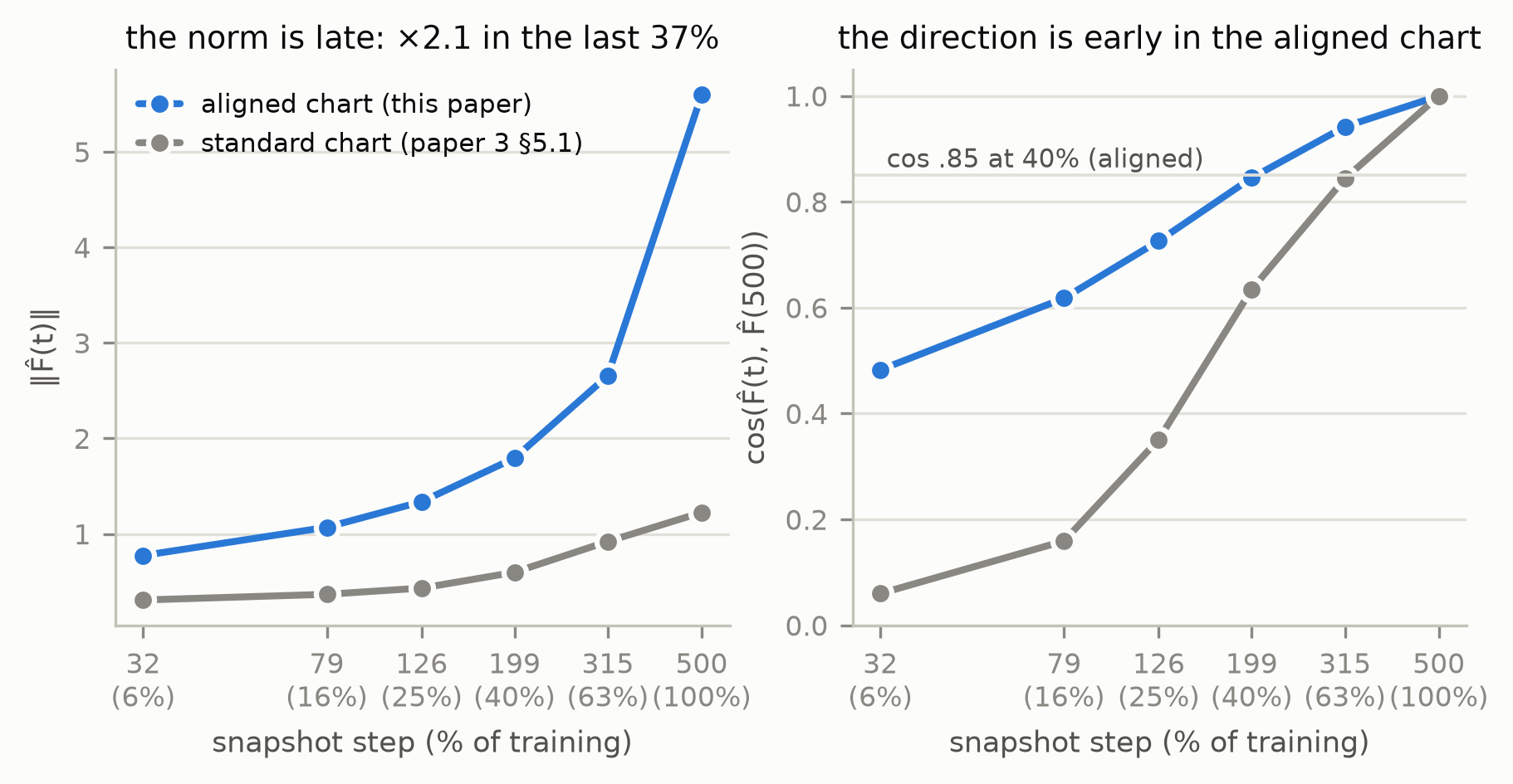
step (% of training)	32 (6)	79 (16)	126 (25)	199 (40)	315 (63)	500 (100)
‖F̂(t)‖, aligned	0.774	1.069	1.337	1.793	2.655	5.597
cos(F̂(t), F̂(500)), aligned	.483	.618	.726	.845	.942	1
A-side / B-side cosine	.237 / .527	.414 / .657	.587 / .756	.781 / .862	.916 / .949	1 / 1

The direction is early and the norm is late. The standard-chart curve is not wrong; it is the curve of a mean that the sign classes annihilate (paper 4 §5.1, |cos| .094 between self-consistent gauges), and its late rise is the rise of whatever survives annihilation. In the aligned chart the mean’s direction is half-set at 6% of training and .85-set at 40%, while its norm grows convexly in log-step and doubles in the final 37%. The B-side cosine leads the A-side at every snapshot, the diagnostic half of the init-subtraction letter (§5.5), which holds. Two rows the table does not show, banked at the audit (p02b-member-trajectory.json): the members’ own RMS norm is 9.0 / 10.3 / 11.2 / 12.4 / 14.1 / 16.2 at the same snapshots — 56% of final at 6%, 77% at 40% — so the coherence ‖F̂‖²/E‖x‖² runs .007 at 6%, .021 at 40%, .035 at 63% and .119 at the end, and the members’ build-time accuracy is .788 / .808 / .816 / .824 / .832 / .840 (medians over all 1,024), within 2 points of final by 40%. Everything below is a consequence of this table: the members are competent early and individually nearly done by 40%; the population has not yet agreed.

5.2 The law is available from 6% of training (P-P02b-2, CONFIRMED 10/10)

ORACLE-MEAN-t renders the banked final mean with the per-block variance table fitted on the step-t snapshots. It is anchor grade at every t including t = 32 — accuracy .820–.824, 63–64 of 64 α-passers, φ 1.0, on both shells (10 registered cells, 10 confirmations; Figure 22). The render-relevant second moment of this population is fixed by 6% of training, and the entire cost of earliness is the mean field.

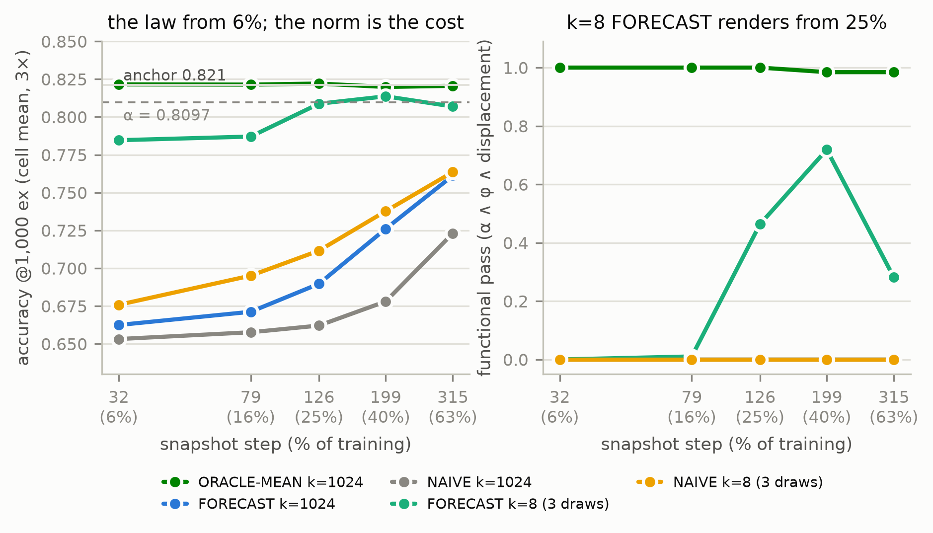
5.3 The naive description and the log-step forecast are dead through 63% (P-P02b-1, P-P02b-3, FALSIFIED)

NAIVE-t, the description fitted on the step-t snapshots of all 1,024 lineages, renders zero α-passers at every t ≤ 315 on both shells (accuracy .653 / .658 / .662 / .678 / .723 at 3×); the registered prediction that it would be anchor grade by 63% fails. FORECAST-t, the untuned log-step extrapolation, beats NAIVE at every t (+1 to +5 points, .662 → .761) and renders zero passers everywhere; the prediction that it would move t* to ≤ 40% fails. Render accuracy tracks the aligned mean’s norm along the trajectory (0.77 → 2.66 of 5.60), not its direction (.48 → .94), and the forecast’s norm reaches only 1.6 → 3.4 with cosine .47 → .95: the direction is nearly right and the magnitude is not, and no line through three earlier points reaches a curve that is convex in log-step. The pre-stated falsification reading applies: the mean’s late component is not log-linearly forecastable in this chart. (Sampling error plays no part in either result: at k = 1,024 the fit is exact to the population; the gap is bias in the dynamics.)

5.4 Task conditioning is present in structure, not at the letter (P-P02b-4, FALSIFIED)

Population B’s forecast is not anchor grade at 25% (0/64); the registered letter fails. But its forecast sits within ~7 points of α at every t against 5–15 for BoolQ’s forecast, and at t = 32 it overshoots the population’s norm (10.85 vs a raw k = 16 mean norm of 7.68; 6.36 k-corrected) and yields 5 of 64 φ-distinct passers — the first hint, on the record before any of §6–§7 fired, that overshoot rather than t gates the render.

5.5 The init-subtraction arm is void at its own gauge check (P-P02b-6, VACUOUS)

The arm was built to test whether the mean’s lateness is the init: remove each member’s init realization by a gauge map in the canonical chart, describe, and add a fresh init back at render. Its registered vacuity guard — the arm’s anchor must reproduce the naive anchor — failed at any tolerance (0/64 vs 64/64; Addendum A), and the arm was voided before a single early-t cell fired, saving ~830 evaluations. The construction is ill-posed in the canonical chart: for three members at t = 500 (Addendum A), ‖A* − g·A(0)‖/‖A*‖ = .37–.39 — the gauge-mapped init carries ~85% of the canonical A-side’s energy, because in LoRA the learned content is expressed within the init’s row space; subtracting the init removes the mean. The well-posed form of “remove the init realization” is the description’s own F̂/E split (paper 3 §5.3), under which the arm is NAIVE. The diagnostic half of the letter (B-side cosine leads A-side at every t ≤ 40%) holds at gate 0 and is reported as a measurement.

5.6 The BALL control is violated at 63% (guard)

A white-noise ball at the step-t law around ONE lineage’s forecast — the Zeng-style control, registered to hold ≤ .10 functional pass at every t — was rendered at three of its five registered t (at 6% and 16% the single forecast row’s own corpus displacement exceeded τ3×, so the shell was unreachable and the cells were recorded, not rendered). It holds at 25% and 40% (0/64 each) and is violated at 63%: 27 of 64 α-passers, φ .963, functional pass .406, where the population forecast at the same t renders none. Registered consequence: the FORECAST-t315 k = 8 cells are flagged as not attributable to the population description, and the flag was applied (§5.7). The reading, labeled: a lineage’s own norm is most of the way to its final well before the mean’s is (§5.1: 77% of final at 40% against the mean’s 32%), so what grows late is chiefly the population’s directional coherence rather than member magnitude — the along-training form of Model Stock’s observation that seed-varied fine-tunes’ pairwise angle decreases steadily with training; the single lineage’s forecast has norm 25.8 / 23.2 / 19.8 at 25% / 40% / 63% against its own final 16.1 (+60% / +44% / +23%), and it renders only at the smallest of those overshoots.

5.7 k does not compound at the letter, and the 8-member forecast renders from 25% (P-P02b-5, CONFIRMED; the surprise)

The letter — t*(k = 8, pooled over three draws) equals t*(k = 1,024) for both arms at 3× — is CONFIRMED as an equality of two right-censored values: nothing reaches ≥ 90% functional pass by 63% at either k. Beneath the letter the arms diverge (Figure 22, right). NAIVE at k = 8 mirrors NAIVE at k = 1,024 (0 passers everywhere; accuracy 2–6 points higher). FORECAST at k = 8 renders working, on-shell, φ-distinct adapters from 25% of training — pooled 3× functional pass .464 (25%) / .719 (40%) / .281 (63%), single-draw 2× .031 / .938 / .156, per-draw range 2–62 of 64, φ = 1.000 among passers, every render on the registered shell — where FORECAST at k = 1,024 renders 0/64 at every t. Its accuracy plateaus at .80–.82 from 25% onward (α = .8097; the k = 8 anchor sits at .82–.83), so cell pass fractions swing on sub-point movements of the mean: not anchor grade, but not dead.

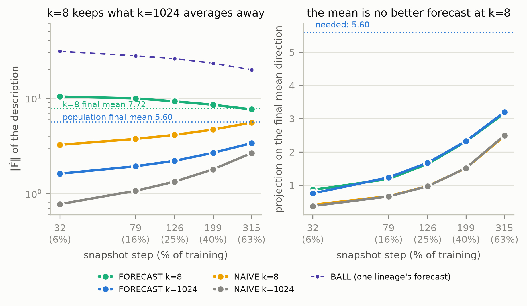
The fit geometry (Figure 23; p02b-fit/*.json, labeled post-hoc) says what the 8-member forecast has that the 1,024-member forecast lacks, and it is not a better mean. The k = 8 forecast’s projection on the population final mean equals the k = 1,024 forecast’s at every t (2.3 at 40% against 5.6 needed). What it carries in addition is ~8 units of norm outside that direction — a 1/√8 superposition of the eight members’ extrapolated residual trajectories (total norm, mean over three draws, 10.4 at 6% → 8.5 at 40% → 7.6 at 63%, against the k = 8 final mean’s 7.72) — which averaging 1,024 forecasts destroys (norm 1.6 → 3.4). That residual is not a forecast of the draw’s own final residual (cosine .03 → .28), and the passers are clones of nothing (φ 1.0). Onset tracks norm overshoot against the own-k final norm, not t: +34% (0), +29% (.01), +20% (.46), +10% (.72), −1% (.28) for the k = 8 forecast; the single-member ball +44% (0) vs +23% (.41); the k = 1,024 forecast undershoots by 40–70% at every t and never renders. Two readings survived this campaign, and they could not both be right: either the mean’s direction is the load-bearing object and the 1,024-member forecast lacked only magnitude, or the 8-member forecast’s off-mean content is functional in its own right. The next campaign was registered to decide between them.

6. The discriminator — direction plus magnitude, or structured residual (P02b-D)

Design. Nineteen cells at 3×, one fire group, registered with a pre-stated framing rule for rung (c). NORMCAL: a banked k = 1,024 direction — FORECAST-t at every t, NAIVE-t at three t, and the final mean itself as the gate-2 anchor — rescaled to the oracle norm 5.5968 and rendered with the early (NAIVE-t) law; nine cells spanning cosine .47 to 1.0. RANDOM: isotropic and block-profiled Gaussian directions at the same norm and law (four cells). K8RESID: the k = 8 forecast and the k = 8 final mean with their projections on the final-mean direction removed, rendered with their own laws (six cells). Calibration placed every norm-5.6 centre, random ones included, at the same corpus displacement (7.9–8.1); among the cells that share the t199 law — the anchor, the two t199 directions and the four random directions — the noise scale was the same as well (c ≈ 1.75), so within that subset direction was the only variable. The other NORMCAL cells carry their own NAIVE-t law (c from 1.55 at t = 315 to 2.40 at t = 32) with the shell held fixed by calibration.

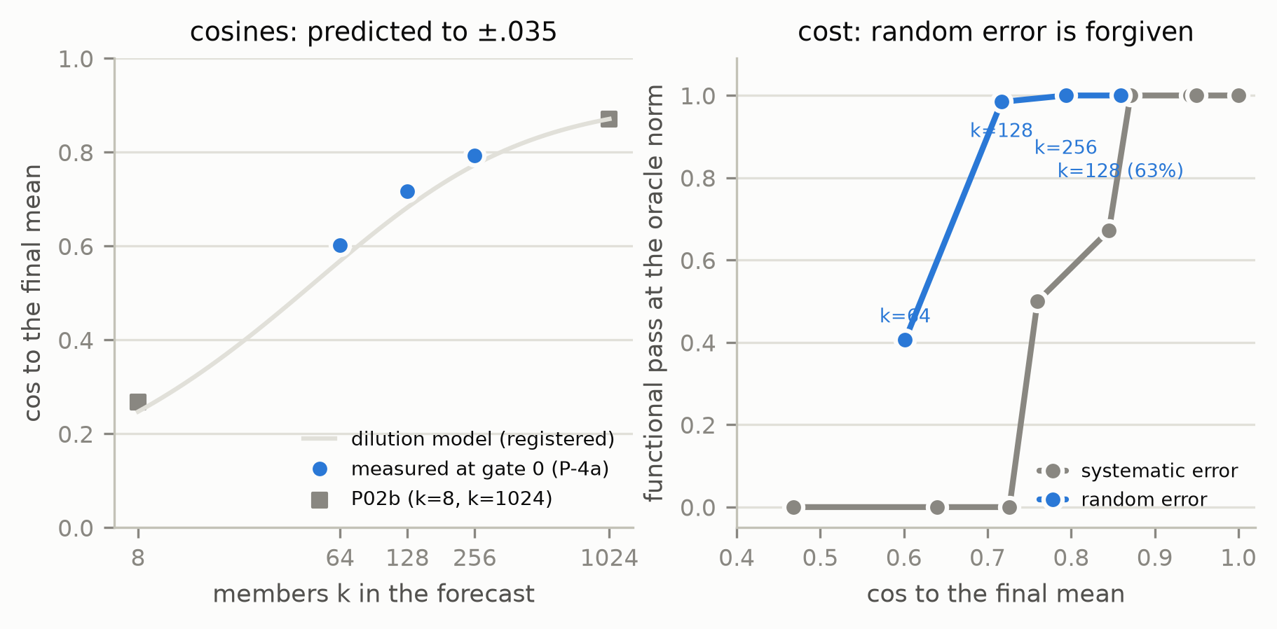
Letters. Gate 2 PASS (anchor 64/64). D-1 CONFIRMED: the k = 1,024 FORECAST-t199 direction, cosine .87, rescaled to the oracle norm, is anchor grade — functional 1.000, accuracy .822 ± .001, φ 1.0; the bar was .50. D-2 CONFIRMED: at fixed norm the render is monotone in direction quality with no inversions — cosine .47 / .64 / .73 → 0; .76 → .50; .85 → .67; .87 / .94 / .95 / 1.0 → 1.000 (accuracy .650 / .780 / .773 / .810 / .813 / .822 / .823 / .823 / .821; Figure 24). The switch-on lies between cosine .73 and .87 — about 40° from the final direction at the half-pass point (cosine .76) and about 30° at full switch-on. D-3 HOLDS: all four random directions at the oracle norm render the base model (0/64, accuracy .648–.650). D-4 CONFIRMED: the residuals alone do not render — the k = 8 forecast residual .021 pooled (0 / 3 / 1 of 64), the real k = 8 final residual .000.

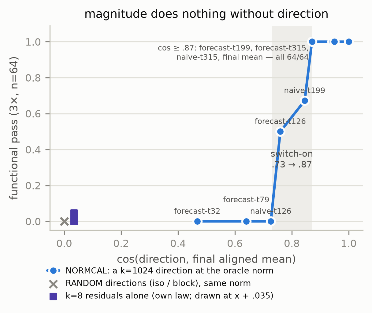
Reading (M), by the pre-stated rule. The mean’s direction is the load-bearing object of the description; it is forecastable at 40% of training; and the entire failure of the 1,024-member forecast in §5.3 was one scalar. Magnitude does nothing without direction (D-3), and the 8-member forecast’s off-mean content works only in combination (D-4). Paper 3’s mechanism narrative — mean plus law — is restored and sharpened: the direction is available early, the norm is not. One side finding, labeled: the extrapolated k = 8 residual alone reaches accuracy .80 (0–3 of 64 passers) while the real k = 8 final residual reaches .67 — the per-member log-step extrapolation concentrates member-specific learned content, which is why it helps the 8-member route and does not, by itself, render.

7. Rung (c) — the norm scalar (P02c)

7.1 The scalar is nearly a constant of the base model, and its block profile is shared

With the k-member inflation removed (‖μ‖² = ‖F̂_k‖² − s²/k; §3), the aligned mean’s final norm across P01’s six strata is (Figure 25):

stratum	‖F̂₁₆‖ raw	‖μ‖ corrected	member norm	coherence ‖μ‖²/E‖x‖²
BoolQ r4 / r8 / r16	6.13 / 7.03 / 8.25	5.47 / 5.94 / 6.40	12.4 / 16.2 / 21.8	.196 / .135 / .087
AG News r4 / r8 / r16	5.57 / 6.51 / 7.68	5.04 / 5.70 / 6.36	10.8 / 13.9 / 18.4	.218 / .169 / .120

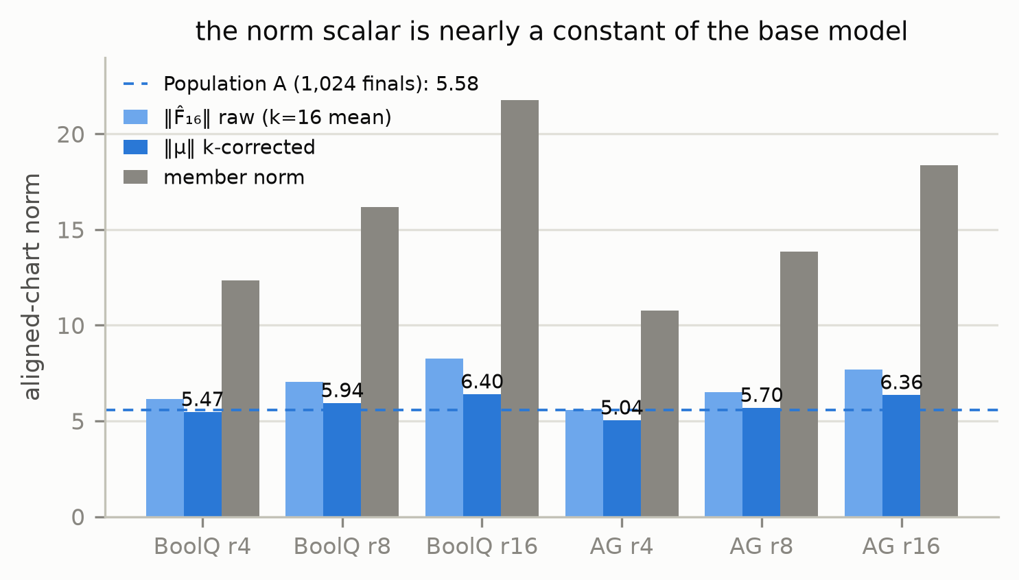
A spread of 5.04–6.40 (mean 5.82) — from +0.46 (BoolQ) to +0.66 (AG News) per rank doubling and a task gap of ≤ 0.44 at fixed rank — while member norms vary twofold and coherence 2.5-fold; Population A’s own value is 5.58. The 196-vector of per-block mean-field norms has cosine ≥ .997 between strata of the same task at adjacent ranks and ≥ .93 across tasks (every pair ≥ .93; banked as p02c-strata-profile.json): the block profile is shared within a task and nearly so across tasks — paper 4’s co-centering finding in norm form. The scalar the trajectory does not supply is, to first order, a property of the base model and recipe, and a transferred norm can be one number. Both qualifiers are load-bearing: task-vector norm disparity is a named failure mode of merging in full-fine-tuning suites with uncontrolled recipes (DisTaC, arXiv:2508.01148), and LoRA’s update magnitude is rank-stable only under the α/√r scaling (rsLoRA, arXiv:2312.03732), so constancy across ranks is a statement about this recipe’s scaling, not about LoRA in general.

7.2 Tolerance is asymmetric: fatal below, free above (P-P02c-1, FALSIFIED on its −15% clause only)

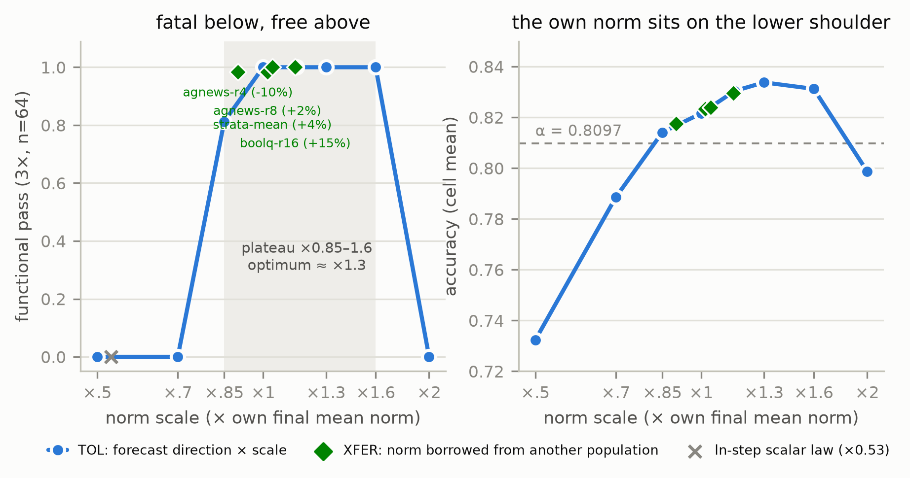
At fixed direction (the k = 1,024 FORECAST-t199, cosine .87) and the early law, scaling the norm across ×{0.5 … 2.0} of the oracle value 5.5968 gives (Figure 26): ×0.50 → 0 (accuracy .732), ×0.70 → 0 (.789), ×0.85 → .812 (.814), ×1.00 → 1.000 (.822), ×1.15 → 1.000 (.830), ×1.30 → 1.000 (.834), ×1.60 → 1.000 (.831), ×2.00 → 0 (.799). The registered ±15% symmetry prediction fails on its low clause (.812 against .90) and holds on its other three. The render plateau runs from ×0.85 to ×1.6 with its optimum near ×1.3; the cliff is between ×0.7 and ×0.85; the turnover is before ×2. The population’s own mean norm sits on the lower shoulder of the render plateau, not at its centre (a reading of the registered curve, labeled) — a borrowed norm need only be at or above it. The nearest published cousin is a gradient-free random-perturbation search result on language models (arXiv:2608.01624) in which the perturbation norm is “the one factor with a failure mode” with a usable range that closes within a factor of five and stays flat inside — same sign, different object, no target direction.

7.3 The norm transfers (P-P02c-2, CONFIRMED — the headline)

The same direction rendered at four norms borrowed from other populations’ k-corrected finals (offsets relative to Population A’s unbiased norm 5.577): AG News r8 (+2.1%) .984, BoolQ r16 (+14.8%) 1.000, AG News r4 (−9.7%, a different task and rank) .984, the six-strata mean (+4.3%) 1.000 — accuracies .823 / .830 / .817 / .824, φ 1.0, every render on shell. A random direction at the transferred norm renders the base model (guard, .650). With §7.6: the description of this population at 40% of its training uses none of its finals — the direction and the law come from its own early snapshots, and the norm from any prior population of the base model and recipe.

7.4 The registered scalar law on the early trajectory does not supply the norm (P-P02c-3, CONFIRMED)

The OLS-in-ln(step) forecast of ln‖F̂(s)‖ over steps 79–199 predicts 2.96 (×0.53); rendered, it gives 0/64 (accuracy .744). Provenance is transfer, not extrapolation; the candidate mechanism — the coherence emerges as the learning rate anneals — needs populations trained under different schedules and is the registered next experiment (§11).

7.5 Random direction error is forgiven; systematic error is not (P-P02c-4, FALSIFIED upward; P-P02c-4a CONFIRMED)

The dilution model predicted the cosine of the k-member forecast to the final mean to within .035 at every k (measured .601 / .717 / .794 at k = 64 / 128 / 256 at 40%, .859 at k = 128 at 63%, against .569 / .683 / .773 / .849) and mispredicted what those cosines cost. At the oracle norm, with the 1,024-member t199 law, the k = 64 direction (cosine .60) renders .406 — the letter’s ≤ .10 clause fails — k = 128 (.72) renders .984, k = 256 (.79) 1.000, and k = 128 at 63% (.86) 1.000; the discriminator’s early-mean directions at cosine .64 and .73 rendered nothing (Figure 27). Cosine to the target is not a sufficient statistic for the render (a reading, labeled): a 1/√k superposition of member residuals around the right direction costs far less than an early mean pointing the wrong way. The member floor for anchor grade at 40% of training is ≤ 128.

7.6 The recipe at k = 256, and the 8-member route’s death by rescale (P-P02c-5 CONFIRMED; P-P02c-6 FALSIFIED)

The (M) recipe — direction from 256 members’ t199 forecasts, law from the same members’ t199 snapshots, norm = the strata mean — renders .990 pooled over three draws (64 / 63 / 63 of 64; accuracies .821 / .822 / .820), against 1.000 for the same k with the oracle norm and the 1,024-member t199 law: the borrowed constant and the 256-member law cost nothing. The cheap (R) route — the banked k = 8 forecast (norm 8.5, .719) rescaled to the same-rank donor’s (AG News r8) k-appropriate final-mean norm 7.237 — renders .047 (0 / 8 / 1 of 64, accuracies .794–.803). Read with §7.2 the reason is plain: the registered target lies 15% below the object’s own norm, on the cliff side of the tolerance curve, while the uncalibrated cell’s +10% overshoot was on the favorable side. The pre-stated falsification reading (“limited by the residual’s direction error, not by overshoot”) does not apply as written — the rescale itself did the damage — and the verdict records the contradiction rather than the reading. The closers (§8) test the rescale in the other direction. On rung (c)’s record the cheapest recipe is (M) at k = 128–256 with one constant.

8. The closers — the gauge, and the 8-member route rescaled upward

Design. Eleven cells at 3×, one fire group, registered before any fit (.research/2026-09-18-p02-closers-prereg.md). SELF: the (M) recipe at k = 256 — direction from the members’ log-step forecasts, law from the same members’ snapshots, norm = the six-strata mean — with the sign gauge discovered from the 256 members’ rows at the latest available snapshot by paper 4’s running-mean sign rule (run in two passes), applied to each member’s earlier snapshots; three draws at 40% (gauge from step 199, forecast over {79, 126, 199}) and three at 63% (gauge from step 315). Nothing from Population A’s finals enters these cells: not the gauge, not the norm, not the law. NORMUP: the banked k = 8 forecast (§5.7) rescaled to ×1.3 of the same-rank donor’s k-appropriate norm (9.41; three draws) and to ×1.6 (11.58; one draw), with its own law. An oracle-mean anchor for gate 2. Listed-direction agreement of the self-discovered signs with the oracle gauge, modulo a global sign per direction, was read at gate 0: .674–.675 at 40%, .740–.744 at 63% — no better at k = 256 than rung (b)’s gate-0 diagnostic measured at k = 8 and k = 1,024 (p02b-verdict.json).

Letters (Figure 28; p02x-verdict.json). Gate 2 PASS (64/64, accuracy .820). C-1a CONFIRMED: the self-gauged recipe at 40% renders 64/64 in every draw — functional 1.000 pooled, accuracy .831 / .833 / .831, φ 1.0 — one point above the oracle-gauge recipe at the same k and norm (.821, §7.6). C-1b CONFIRMED: at 63%, 64/64 in every draw (accuracy .829). C-2 CONFIRMED: the k = 8 forecast at ×1.3 renders .984 / 1.000 / .859 (accuracies .818 / .822 / .815), .948 pooled against a .90 bar, from .047 at ×1.0 and .719 uncalibrated; at ×1.6 it renders 1.000 with accuracy .830, the highest of the four NORMUP cells and of any k = 8 cell on record.

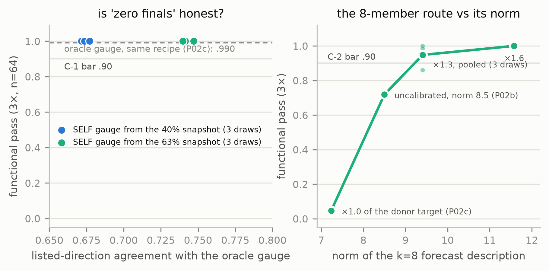
Reading, labeled. (1) “Zero finals” is honest. A gauge that is self-consistent among the 40% rows renders at least as well as the final’s gauge imposed on those rows — better by a point — while agreeing with it on only two thirds of the listed directions. Paper 3’s finding that the SELF gauge does not match the final’s before the end of training was a statement about agreement, and agreement with the final is not what the render needs; self-consistency at t is. Why the self-consistent chart is slightly better than the final’s chart applied early is not answered here. (2) The k = 8 object’s render optimum lies above ×1.3 of its k-appropriate norm (×1.6 is better than ×1.3, and both are far above the ×1.0 that killed it in §7.6) — the same asymmetry as §7.2, shifted higher for a description that carries a 1/√8 residual superposition. (3) The cheapest description on record is eight lineages’ snapshots at 40% of training, a same-rank donor’s two constants, and a ×1.3–1.6 rescale: about 3.2 lineage-trainings-equivalent of compute against paper 4’s eight finished lineages — a 2.5× reduction — at the price of a second borrowed constant and draw dependence (one draw at ×1.3 rendered .859). (4) The top-up discipline earned its keep: the ×1.6 cell read .17 functional — its renders’ φ unscorable — before their single nearest corpus row was banked, and 1.000 after (a hazard now on the lab’s improvements ledger).

9. The description along training: what each phase contributes

Read across the four campaigns (Figure 29), the two-moment description of this population is assembled in three phases with three clocks:

• The law, by 6%. The per-block variance table fitted on the step-32 snapshots renders anchor grade with the final mean (§5.2). What paper 3 called “the law forms early” is early even by the standard of a 500-step run.
• The direction, by 40%. The aligned mean’s direction is .85 to its final at step 199 and .87 under the untuned extrapolation (§5.1, §6); given the norm, the extrapolated direction renders at anchor grade and the raw one renders .67 (§6); from 128 members’ forecasts it is .72 and still renders .98, because the members’ residual error is random around the right direction and the render forgives that kind of error (§7.5).
• The norm, late — and shared. The aligned mean’s norm doubles in the last 37% of training (§5.1), defeats every 1,024-member early description (§5.3), and is not supplied by the registered log-step scalar law (§7.4). It is nearly the same number across six task × rank strata of the base model (§7.1), the render tolerates it from ×0.85 to ×1.6 with its optimum above the population’s own value (§7.2), and every borrowed value rendered anchor grade (§7.3). Members’ norms grow ×1.8 from 6% to 100% of training and their accuracy is near-final by 40% (§5.1); the mean’s norm grows ×7; what grows late is chiefly their agreement. Seen through the description, the late phase of training is a one-scalar coherence event.

The practitioner recipe, v2. Paper 4’s five clauses stand (one registered sign anchor; ≥ 8 members per stratum for a description from finals; rank high enough for coverage; render depth as a task-conditioned absolute budget; the functional filter non-optional). This paper adds when: (f) a population’s description can be taken at 40% of its training from ≥ 128–256 lineages’ snapshots — three snapshots per lineage for the extrapolation, the latest for the law (128 measured for the direction alone — oracle norm, 1,024-member law; 256 with the borrowed norm and the members’ own law); (g) the norm is not in the snapshots — borrow it from any prior population of the same base model and recipe, k-corrected, and take it at or above the population’s own value where possible: relative to the oracle norm, −10% still rendered .984, −15% is the plateau’s lower edge where a fifth of renders fail, the cliff lies between −30% and −15%, and the plateau runs to +60%; (h) the sign gauge can be discovered from the same 40% snapshots by the running-mean sign rule (§8; measured at k = 256): no final of the described population enters; (i) the cheapest form is eight lineages’ snapshots at 40% plus a same-rank donor’s ‖μ‖ and s², the forecast rescaled ×1.3–1.6 above the k-appropriate norm and never below (§8; rendered in the finals’ gauge — the self-discovered gauge of (h) was not tested at k = 8) — about three lineage-trainings of compute for an anchor-grade description.

What this does not say. Not that individual partially trained adapters are useless — they are near-final by 40% (§5.1) — nor that their raw mean is useful: it renders nothing. Not that the 256-lineage form saves training compute: it consumes 256 lineages at 40% each against eight finished lineages for paper 4’s route, and its cheapness is that no run has to finish, that a population can be described before its training campaign ends, that abandoned or partial runs become usable data, and that the norm is reusable across populations. The eight-lineage form (§8) does save compute — 3.2 lineage-trainings against eight — at the price of a second borrowed constant and a same-rank donor. And not that learning has lost ground: steering, and everything past the full-network basin edge, are where paper 4 left them.

10. Limitations

Regime-boundedness. One base model (Qwen3-0.6B, revision-pinned); every render of the discriminator and rung (c), and every Population-A render, is BoolQ at rank 8 on a seed-pure population; AG News r16 was rendered only in rung (b)’s task-conditioning cells (ten registered, seven fired; §5.4) and otherwise appears, with the other five P01 strata, as a norm donor. One snapshot schedule (eleven log-spaced steps of a 500-step run) and one learning-rate schedule — the candidate mechanism for the late coherence (§7.4) is untested and is the registered next experiment. One forecaster, deliberately untuned; a tuned or mechanism-aware forecaster might move the direction’s clock earlier; the one registered scalar law did not move the norm’s (§7.4), and whether any smooth law could is untested.

The gauge. Every description in §5–§7, and the 8-member route of §8, is in the oracle-aligned chart: each member’s sign pattern from its final, applied to its snapshots. “Zero finals” in §7.3 and §7.6 is therefore zero finals for the description’s two moments; the alignment used the finals. Rung (b)’s gate-0 diagnostic found the SELF gauge does not match the final’s before the end of training (listed-direction agreement .58–.74 at ≤ 63% for k = 8 and k = 1,024, .996 at 100%; p02b-verdict.json); the closers measured the consequence directly and found none — the self-consistent gauge at 40% renders at least as well (§8) — so the asterisk is removed for this population, with the same regime bounds as everything else here. Under Saravanan and Salla’s result (§2) any self-discovered gauge is conditional on distance from the collision strata; our populations are not on them, and the ill-conditioning is measurable per block, which this paper does not do.

Resolution and single-direction curves. The two tolerance curves (§6, §7.2) are nine points each, on one population, and the norm curve uses one direction; the direction-economics cells are single draws (the k = 256 direction is replicated in three draws only in the recipe cells of §7.6). A 64-render cell resolves pass fractions at roughly ±0.12 (2σ at p = .5), and a cell whose mean sits on the α bar swings its pass fraction on sub-point movements (the hazard noted in §4); the letters were set at .90 / .50 / .25 / .10 for that reason and the decisive cells sit at 63–64 or 0–8 of 64, but the ×0.85 cell’s .812 and the k = 64 cell’s .406 are readings near the steep part. The k-correction’s small-k variance is bootstrapped on Population A’s Gram and assumed for the donors.

The donors. All six come from one harvest with one recipe; the “constant of the base model” reading (§7.1) is six points on two tasks and three ranks. Transfer from a population trained under another recipe, another base, or a harvest of unknown provenance is not measured.

φ and the audit. As throughout the series, φ with i.i.d. probes is a lower bound on functional distinctness; no claim concerns rendered adapters beyond the audited task; the hubness hygiene check on nearest-neighbor novelty remains logged and unrun.

Post-hoc readings. The fit-geometry reading of the 8-member surprise (§5.7), the coherence reading of the BALL violation (§5.6), the “lower shoulder” reading of the tolerance curve (§7.2), and the random-vs- systematic error reading (§7.5) are labeled post-hoc readings of registered numbers; the discriminator converted the first into a registered test, and the others are candidates for the same.

11. Discussion

The series’ through-line, extended once more. Paper 1: fixing the coordinates makes honest generation possible. Paper 2: the frontier belongs to operators that respect the population’s geometry. Paper 3: with the coordinates fixed, the density that remains is a mean and a variance table. Paper 4: that description is estimable from eight members, in a gauge the estimator can discover itself, and bounded by regime, task, rank and gauge discipline. This paper: the description is present in the members’ trajectories at 40% of training except for one scalar, and that scalar is a property of the base model and recipe rather than of the population. Three morals seem worth stating.

Describe-before-the-end is a population property, not a checkpoint property. Individual early adapters are near-final in accuracy by 40%, yet no raw mean of early snapshots renders; what the early trajectory carries is a direction that only averaging many members’ extrapolations reveals, and the render forgives the residual of that average because it is random. The law of large numbers is the cost of the recipe, not its content — the content is that the population’s direction stops rotating well before its members stop moving.

Cosine to the target is not a sufficient statistic for a render. Two directions at nearly the same cosine to the final mean (.72 and .73) rendered .98 and 0 (§7.5), and the difference was the kind of error: random member residuals around the right direction against an early mean pointing the wrong way. Every audit in this series that scored geometry against function found geometry insufficient; this is the version for directions, and it is the reason the member floor at 40% is at most 128 (the 64-member direction already renders .41) where the dilution model’s switch-on cosine would have asked for about 1,000 (§3).

The late phase of training is, at the population level, a scalar coherence event. Members are near-final in accuracy by 40% and their norms grow only ×1.8 from 6% to 100% of training while the mean’s grows ×7; what changes in the last 37% of training is chiefly their agreement, and the amount of it is nearly the same across tasks and ranks of the base model. That is a statement about what training does, made through the description rather than through any single trajectory, and it points at the next experiment: whether the coherence tracks the learning-rate anneal. If it does, the one number the recipe borrows is a property of the recipe, not of the task — and a population’s description at 40% of its training is then, in every part, available before the population is.

The open questions are specific. The schedule experiment above. Why a sign gauge that agrees with the final’s on only two thirds of the listed directions renders a point better than the final’s gauge applied to the same rows (§8) — the closers removed the asterisk and posed the question. Why the render optimum sits above the population’s own norm at ×1.3 — a question about the task function’s landscape that the tolerance curve poses and nothing here answers. And the program-level consequence: the description’s expensive part is task-independent and its task-dependent part is a direction that paper 4 located in a few late-layer blocks, so a map from a task to a description has only a direction to produce — the series’ original destination, narrowed to its actual size.

12. Reproducibility statement

Four pre-registrations, frozen before firing, with their decision logs and addenda: .research/2026-09-14-p02b-prereg.md (v1 + Addendum A), .research/2026-09-16-p02bd-prereg.md, .research/2026-09-17-p02c-prereg.md, .research/2026-09-18-p02-closers-prereg.md. Toolchain: p02b_run.py / p02b_popb.py / p02b_selfdiag.py / p02b_verdict.py, p02bd_run.py, p02c_run.py, p02x_run.py, each with its drive script; every cell regenerates from its banked manifest and calibration; every verdict JSON is written mechanically by the assembler from the stats files, with labeled post-hoc fields. Artifacts of record: the verdict, stats, gate, calibration and constants JSONs (p02b-verdict.json, p02b-stats.json, p02b-popb-stats.json, p02b-et.json, p02b-gate0-report.json, p02b-gate2-report.json, p02b-member-trajectory.json, p02bd-verdict.json, p02bd-stats.json, p02bd-gate0.json, p02c-verdict.json, p02c-stats.json, p02c-gate0.json, p02c-calibration.json, p02c-constants.json, p02x-verdict.json, p02x-stats.json, p02x-gate0.json, p02x-calibration.json); the fit sidecars (p02b-fit/*.json, p02bd-fit, p02c-fit, p02x-fit) carrying every description’s norm and cosine; the aligned-finals Gram (p02c-gram-finals-aligned.npy) and the k-correction bootstrap. Figures 21–29 are generated from these artifacts, and the strata-survey figure also from P01’s six stratum descriptions (p01-fit/s0..s5-D.npz), by scripts/make_figures.py. Journal entries 122–137 on thread 2f020918 carry each campaign’s tables and labeled readings; the KB articles research.xaos.findings.p02b (rev 4) and research.xaos.findings.p02c (rev 2) are the findings of record. Pre-publication: two numbers-vs-artifacts audits, an internal-consistency audit, a citation re-walk primary-verifying every reference below, and a final whole-document validation of the pinned bundle by four independent read-only agents (427 items traced; every finding applied), all on the record before publication.

References

(Items marked ◆ carry over from the verified bibliographies of papers 1–4; items marked ▸ are new to the series, located by the 2026-09-14 field sweep and the 2026-09-18 scoop sweep. Every entry below was primary-verified against its arXiv, proceedings or publisher record in the pre-publication re-walk.)

The series

1. Canonicalize, Then Generate. Haphazard Solutions lab publication, 2026. haphazardsolutions.com/knowledge/canonicalize-then-generate/.
2. Recombine, Then Generate. Haphazard Solutions lab publication, 2026. haphazardsolutions.com/knowledge/recombine-then-generate/.
3. Describe, Then Render. Haphazard Solutions lab publication, 2026. haphazardsolutions.com/knowledge/describe-then-render/.
4. Describe from Little, in Any Gauge. Haphazard Solutions lab publication, 2026. haphazardsolutions.com/knowledge/describe-from-little-in-any-gauge/.

Population statistics from partially trained members

1. ▸ Hirst, Ramgoolam. Approximate Gaussianity Beyond Initialisation in Neural Networks. arXiv:2510.05218 (2025). — a permutation-invariant Gaussian matrix model fitted to a 1,000-member ensemble at every epoch; never sampled.
2. ◆ Schürholt, Knyazev, Giró-i-Nieto, Borth. Hyper-Representations as Generative Models: Sampling Unseen Neural Network Weights. NeurIPS 2022. arXiv:2209.14733. — fit at epochs 21–25, “not fully converged.”
3. ◆ Schürholt, Mahoney, Borth. Towards Scalable and Versatile Weight Space Learning (SANE). ICML 2024. arXiv:2406.09997. — first-half-epochs training; the Gaussian variant fails zero-shot.
4. ◆ Peebles, Radosavovic, Brooks, Efros, Malik. Learning to Learn with Generative Models of Neural Network Checkpoints (G.pt). arXiv:2209.12892 (2022).
5. ▸ Tang et al. Predicting Mergeability of Parameter-Efficient Fine-Tuning Updates (MergeProbe). arXiv:2606.19549 (2026). — an early-training population scalar.
6. ◆ Han et al. A Survey of Weight Space Learning: Understanding, Representation, and Generation. arXiv:2603.10090 (2026). — no section on population-statistic estimation.
7. ◆ Z. Wang, P. Wang, K. Wang. Position: Weight Space Should Be a First-Class Generative AI Modality. ICML 2026 (Position Paper Track). arXiv:2605.18632.

When the outcome is pinned

1. ▸ Frankle, Schwab, Morcos. The Early Phase of Neural Network Training. ICLR 2020. arXiv:2002.10365.
2. ◆ Frankle, Dziugaite, Roy, Carbin. Linear Mode Connectivity and the Lottery Ticket Hypothesis. ICML 2020. arXiv:1912.05671.
3. ▸ You et al. Drawing Early-Bird Tickets: Towards More Efficient Training of Deep Networks. ICLR 2020. arXiv:1909.11957.
4. ◆ Gur-Ari, Roberts, Dyer. Gradient Descent Happens in a Tiny Subspace. arXiv:1812.04754 (2018).
5. ▸ Sakai, Ichikawa. Sign Lock-In: Randomly Initialized Weight Signs Persist and Bottleneck Sub-Bit Model Compression. ICML 2026. arXiv:2602.17063.
6. ▸ Jastrzębski et al. The Break-Even Point on Optimization Trajectories of Deep Neural Networks. ICLR 2020. arXiv:2002.09572.
7. ▸ Achille, Rovere, Soatto. Critical Learning Periods in Deep Networks. ICLR 2019. arXiv:1711.08856.
8. ▸ Kwok, Altıntaş, Raffel, Rolnick. The Butterfly Effect: Neural Network Training Trajectories Are Highly Sensitive to Initial Conditions. ICML 2025. arXiv:2506.13234.
9. ▸ Yang, Shi, Hu, Xing, Liu. Robustness Emerges Early in Training Dynamics, but Is Not Preserved. ECCV 2026. arXiv:2608.04442.

Spectral laws over training; LoRA timing

1. ▸ Zhang, Liu, Chen. LoRA-One: One-Step Full Gradient Could Suffice for Fine-Tuning Large Language Models, Provably and Efficiently. ICML 2025 (Oral). arXiv:2502.01235.
2. ▸ Zhang, Zhou, Jia, Chen, Cheng. The Stability of Singular Distribution: A Spectral Perspective on the Two-Phase Dynamics of Language Model Pre-training. arXiv:2605.26489 (2026).
3. ▸ Piontkovskaia, Nikolenko. Recoverable but Not Stationary: Local Linear Structures in Weights and Activations. arXiv:2606.10929 (2026).
4. ▸ Sato, Tanaka, Nakamura, Kobayashi, Ito. Behaviorally Effective LoRA Writes Are Sparse and Structured. arXiv:2609.01374 (2026).
5. ▸ Park, Bocchi, D’Amico, Lucini, Aarts. Spectral Phase Transitions and Trainability in Neural Network Learning Dynamics. arXiv:2606.28486 (2026).
6. ▸ Lauditi, Pehlevan, Bordelon. Spectral Dynamics in Deep Networks: Feature Learning, Outlier Escape, and Learning Rate Transfer. arXiv:2605.07870 (2026).
7. ▸ Saxe, McClelland, Ganguli. Exact Solutions to the Nonlinear Dynamics of Learning in Deep Linear Neural Networks. ICLR 2014. arXiv:1312.6120.
8. ▸ Yaras, Wang, Balzano, Qu. Compressible Dynamics in Deep Overparameterized Low-Rank Learning and Adaptation (Deep LoRA). ICML 2024 (Oral). arXiv:2406.04112.
9. ◆ Guth, Ménard, Rochette, Mallat. A Rainbow in Deep Network Black Boxes. JMLR 25 (2024). arXiv:2305.18512.
10. ◆ Martin, Mahoney. Implicit Self-Regularization in Deep Neural Networks. JMLR 22 (2021). arXiv:1810.01075.
11. ▸ Zhuang et al. Come Together, But Not Right Now: A Progressive Strategy to Boost Low-Rank Adaptation (CoTo). ICML 2025. arXiv:2506.05713.
12. ▸ Wu, Gao, Li, Wu. Stable-LoRA: Stabilizing Feature Learning of Low-Rank Adaptation. ICLR 2026. arXiv:2603.05204.

Task-conditioned adapter generation

1. ▸ Li, Chen, Rao, Jiang, Guo. Semantic-Guided LoRA Parameters Generation (SG-LoRA). arXiv:2509.10535 (2025). — a learned generator from task descriptions; no notion of adapter norm.
2. ▸ Soro et al. Diffusion-Based Neural Network Weights Generation (D2NWG). ICLR 2025. arXiv:2402.18153.
3. ▸ Asefaw, Tzevelekakis, Falk, Meynent, Borth. WeightCLIP: Aligning Datasets and Models for Weight Space Learning. ICML 2026. arXiv:2607.03551.
4. ▸ Lin, Li, Shen, Liu, Zeng. GME-Init: Gamma-Moment Equalization for LoRA Initialization in Parameter-Efficient Fine-Tuning. Entropy 28(8):873 (2026). — per-layer variance from calibration passes; no mean.
5. ▸ Paischer et al. Parameter Efficient Fine-tuning via Explained Variance Adaptation (EVA). NeurIPS 2025. arXiv:2410.07170.
6. ▸ Das et al. ConsNoTrainLoRA: Data-driven Weight Initialization of Low-rank Adapters using Constraints (CNTLoRA). ICCV 2025. arXiv:2507.08044.
7. ◆ Charakorn, Cetin, Tang, Lange. Text-to-LoRA. ICML 2025. arXiv:2506.06105.
8. ◆ Khan, Tang, Li, Wang, Chen. ORAL. arXiv:2503.24354 (2025).
9. ◆ Huang et al. LoRAGen: Structure-Aware Weight Space Learning for LoRA Generation. ICLR 2026.

Gauge, convention, and replication doctrine

1. ◆ Doyle, Hu, Chan, Leontjeva. Learning Adapter Rank via Symmetry Breaking. arXiv:2506.22809 (2025; Thm 1).
2. ◆ Bro, Acar, Kolda. Resolving the Sign Ambiguity in the Singular Value Decomposition. J. Chemometrics 22(2), 2008.
3. ▸ Karuturi, Bukkapatnam, Patel, Shastry. The GL(r) Gauge Symmetry of LoRA: Principal Bundle Structure, Loss Landscape Geometry, and Implications for Adapter Merging. ICML 2026 Workshop on Weight Space Symmetries.
4. ▸ da Silva, Adnan, Dangel, Oore. Generalizing the Geometry of Model Merging Through Fréchet Averages. arXiv:2604.27155 (2026); and A Geometric View of Model Merging: Quotient Fréchet Averages from Toy Models to LoRA. ICML 2026 Workshop WSS.
5. ▸ Saravanan, Salla. No Global Gauge in Neural Weight Space: Branched Quotient Geometry and Atlas-Optimal Learning. ICML 2026 Workshop WSS.
6. ▸ Kiwitt, Tahmasebi, Jegelka. Symmetries in Weight Space Learning: To Retain or Remove? HiLD Workshop @ ICML 2025.
7. ▸ Ito, Yamada, Chijiwa, Kumagai. Do We Really Need Permutations? Impact of Model Width on Linear Mode Connectivity. ICLR 2026.
8. ▸ Artemev, Xia, Boyd, Yu, Dangel, Hennequin, Bernacchia. Exploiting Weight-Space Symmetries for Approximating Curvature. ICML 2026.
9. ▸ Sweeney. Signed-Permutation Coordinate Transport for RMSNorm Transformers. arXiv:2606.31963 (2026). — explicit-gauge doctrine for RMSNorm, stated before paper 3.
10. ▸ Brömme. Canonicalization Failures as a Recurring Vulnerability Class: Representation Divergence in Cryptographic Systems and Its Avoidance. arXiv:2608.06508 (2026).
11. ◆ Elitzur. Impossibility of Spontaneously Breaking Local Symmetries. Phys. Rev. D 12:3978, 1975.
12. ◆ Gribov. Quantization of Nonabelian Gauge Theories. Nucl. Phys. B 139:1–23, 1978.
13. ◆ Zhao, Walters, Yu. Symmetry in Neural Network Parameter Spaces. TMLR 2025. arXiv:2506.13018.
14. ▸ Xu et al. Quotient-Space Diffusion Models. ICLR 2026 (Oral).
15. ◆ Cain. Gauge Freedom and Metric Dependence in Neural Representation Spaces. arXiv:2603.06774 (2026).

Audit doctrine and instruments

1. ◆ Zeng, Yin, Xu, Liu. Generative Modeling of Weights: Generalization or Memorization? CVPR 2026. arXiv:2506.07998.
2. ◆ Theis, van den Oord, Bethge. A Note on the Evaluation of Generative Models. ICLR 2016. arXiv:1511.01844.
3. ◆ Merger, Goldt. Local Coverage Governs Memorization in Diffusion Models. arXiv:2606.14390 (2026).
4. ◆ Klabunde, Schumacher, Strohmaier, Lemmerich. Similarity of Neural Network Models. ACM Comput. Surv. 57(9), 2025. arXiv:2305.06329.
5. ◆ Cao, Jia, Gong. IPGuard. AsiaCCS 2021. arXiv:1910.12903.
6. ◆ Lukas, Zhang, Kerschbaum. Deep Neural Network Fingerprinting by Conferrable Adversarial Examples. ICLR 2021. arXiv:1912.00888.
7. ◆ Salvy, Talbot, Thirion. GICDM: Mitigating Hubness for Reliable Distance-Based Generative Model Evaluation. ICML 2026. arXiv:2602.16449.
8. ◆ Radovanović, Nanopoulos, Ivanović. Hubs in Space. JMLR 11, 2010.
9. ▸ B. Chen. Token Counts Are Not Model Lineage: A Frozen-Threshold Holdout Study of Black-Box LLM API Fingerprinting. arXiv:2608.29930 (2026).
10. ▸ Cooper. Playing Whack-a-Mole with Misconceptions about Memorization, Extraction, and Copyright. arXiv:2609.09320 (2026).
11. ▸ Thakur, Khoury. Training Leaves Traces: Centered Residual Signatures for Language Model Lineage Verification. arXiv:2608.14929 (2026).
12. ▸ Chen, Shang, Liu. Who Built This Model? Tracing LLM Lineage via Spectral Fingerprints in Weight Space. COLM 2026. arXiv:2608.07786.
13. ◆ Vovk. Conditional Validity of Inductive Conformal Predictors. PMLR 25, 2012.
14. ◆ Angelopoulos, Bates. A Gentle Introduction to Conformal Prediction. arXiv:2107.07511 (2021).

Pre-registration norms

1. ◆ Nosek, Errington. What Is Replication? PLoS Biol. 18(3):e3000691, 2020.
2. ◆ Willroth, Atherton. Best Laid Plans: A Guide to Reporting Preregistration Deviations. AMPPS 7(1), 2024.
3. ◆ Lakens. When and How to Deviate From a Preregistration. Collabra: Psychology 10(1):117094, 2024.
4. ◆ Pascale et al. SN H0pe. ApJ 979(1):13, 2025. arXiv:2403.18902.

Population geometry and task structure

1. ◆ Jang, Yun, Han. Model Stock. ECCV 2024. arXiv:2403.19522.
2. ◆ Wortsman et al. Model Soups. ICML 2022. arXiv:2203.05482.
3. ◆ Hu et al. LoRA: Low-Rank Adaptation of Large Language Models. ICLR 2022. arXiv:2106.09685.
4. ◆ Ilharco et al. Editing Models with Task Arithmetic. ICLR 2023. arXiv:2212.04089.
5. ◆ Gueta et al. Knowledge Is a Region in Weight Space for Fine-tuned Language Models. Findings of EMNLP 2023. arXiv:2302.04863.
6. ◆ Panigrahi, Saunshi, Zhao, Arora. Task-Specific Skill Localization in Fine-tuned Language Models. ICML 2023. arXiv:2302.06600.
7. ◆ Geva, Schuster, Berant, Levy. Transformer Feed-Forward Layers Are Key-Value Memories. EMNLP 2021. arXiv:2012.14913.

Adjacent priors: extrapolation, trajectory dynamics, norm and scale

1. ▸ Zheng, Wang, Ji, Huang, Peng. Model Extrapolation Expedites Alignment (ExPO). ACL 2025. arXiv:2404.16792. — checkpoint extrapolation θ₁ + αΔθ from 10–40% of DPO training, α tuned; sharp drops at large α.
2. ▸ Wang et al. Linear Dynamics in the RLVR Training of Large Language Models. arXiv 2026. arXiv:2601.04537. — per-weight linear regression in step; two-checkpoint extrapolation; inverted-U in the extrapolation ratio.
3. ▸ Wei et al. You Only Need Minimal RLVR Training: Extrapolating LLMs via Rank-1 Trajectories (RELEX). arXiv 2026. arXiv:2605.21468. — rank-1 drift plus regression from a 15% window; magnitude predicted from the trajectory on a single run.
4. ▸ Yoshida, Naraki, Horie, Shimizu, Naganuma. DisTaC: Conditioning Task Vectors via Distillation for Robust Model Merging (DisTaC). arXiv 2025. arXiv:2508.01148. — task-vector norm disparity as a merging failure mode under uncontrolled recipes.
5. ▸ Kalajdzievski. A Rank Stabilization Scaling Factor for Fine-Tuning with LoRA (rsLoRA). arXiv 2023. arXiv:2312.03732. — update magnitude rank-stable only under α/√r scaling.
6. ▸ Kim, Kim, Kim, Lee. Not the Dimension, the Norm: What Matters in Gradient-Free Weight Perturbation of Language Models. arXiv 2026. arXiv:2608.01624. — the perturbation norm as the one factor with a failure mode; a safe range that transfers across scale and family.